Context
Last week, I was discussing about how to use nls() for a specific
model with one of my colleague and I ended creating a piece of code to
show what I was talking about! Even though there are many posts exploring nls()
in more depth that I did (for instance this post on datascienceplus by Lionel Herzog),
I thought I could share these lines of command here!
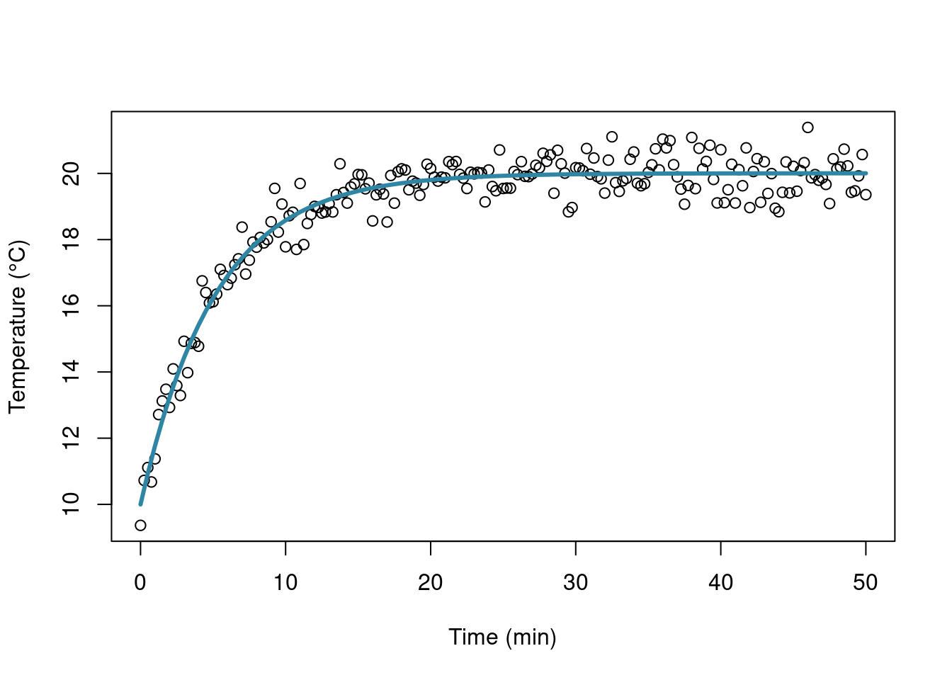
Basically, we were talking about a model where the temperature (\(T\)) follows
a saturation curve starting from 10°C at t=0 (so T(0) = 10) and plateauing at \(T_{\inf}\).
$$T(t) = T_{\inf} - (T_{\inf} - T_0)\exp(-kt)$$
Goal and data
The goal here is to use nls() (Nonlinear Least Squares) to find \(k\) and \(T_{inf}\).
For the sack of clarity, I simulate the data, i.e. I use the saturation curve
with known parameter values, then I add some noise (here a white noise):
 1
 2
 3
 4
 5
 6
 7
 8
 9
10
11
12
13
14
15
16
17
18
19
20
21
22
23
24
|
library(magrittr)
# Parameters
## known
T0 = 10
## the ones we are looking for
k = 0.2
Tinf = 20

# Simulate data
## time
seqt <- seq(0, 50, .25)
## create a data frame
simdata <- cbind(
  seqt = seqt,
  sim = Tinf - (Tinf- T0) * exp(-k * seqt) + .5 * rnorm(length(seqt))
) %>% as.data.frame
head(simdata)
#R>    seqt       sim
#R>  1 0.00  9.303692
#R>  2 0.25 10.745711
#R>  3 0.50 11.112195
#R>  4 0.75 12.195986
#R>  5 1.00 11.064262
#R>  6 1.25 11.510062
|
Use nls()
Now I call nls() to fit the data:
1
|
res <- nls(sim ~ Tinf - (Tinf - 10)*exp(-k*seqt), simdata, list(Tinf = 1, k = .1))
|
All the information needed are stored in res and display via the print method:
 1
 2
 3
 4
 5
 6
 7
 8
 9
10
|
res
#R>  Nonlinear regression model
#R>    model: sim ~ Tinf - (Tinf - 10) * exp(-k * seqt)
#R>     data: simdata
#R>     Tinf       k
#R>  20.0709  0.1938
#R>   residual sum-of-squares: 46.45
#R>
#R>  Number of iterations to convergence: 8
#R>  Achieved convergence tolerance: 2.562e-07
|
Let’s draw a quick plot:
1
2
3
4
5
|
## get the coefficients values
cr <- coef(res)
fitC <- function(x) cr[1] - (cr[1] - 10)*exp(-cr[2]*x)
plot(simdata[,1], simdata[,2], xlab = "Time (min)", ylab = "Temperature (°C)")
curve(fitC, 0, 50, add = TRUE, col = "#2f85a4", lwd = 3)
|
That’s all folks!
Display information relative to the R session used to render this post.
 1
 2
 3
 4
 5
 6
 7
 8
 9
10
11
12
13
14
15
16
17
18
19
20
21
22
23
24
25
26
27
28
29
30
31
32
33
34
|
sessionInfo()
#R>  R version 4.5.1 (2025-06-13)
#R>  Platform: x86_64-pc-linux-gnu
#R>  Running under: Ubuntu 24.04.2 LTS
#R>
#R>  Matrix products: default
#R>  BLAS:   /usr/lib/x86_64-linux-gnu/openblas-pthread/libblas.so.3
#R>  LAPACK: /usr/lib/x86_64-linux-gnu/openblas-pthread/libopenblasp-r0.3.26.so;  LAPACK version 3.12.0
#R>
#R>  locale:
#R>   [1] LC_CTYPE=C.UTF-8       LC_NUMERIC=C           LC_TIME=C.UTF-8        LC_COLLATE=C.UTF-8
#R>   [5] LC_MONETARY=C.UTF-8    LC_MESSAGES=C.UTF-8    LC_PAPER=C.UTF-8       LC_NAME=C
#R>   [9] LC_ADDRESS=C           LC_TELEPHONE=C         LC_MEASUREMENT=C.UTF-8 LC_IDENTIFICATION=C
#R>
#R>  time zone: UTC
#R>  tzcode source: system (glibc)
#R>
#R>  attached base packages:
#R>  [1] stats     graphics  grDevices utils     datasets  methods   base
#R>
#R>  other attached packages:
#R>  [1] magrittr_2.0.3    inSilecoRef_0.1.1
#R>
#R>  loaded via a namespace (and not attached):
#R>   [1] sass_0.4.10       generics_0.1.4    xml2_1.3.8        blogdown_1.21     stringi_1.8.7
#R>   [6] httpcode_0.3.0    digest_0.6.37     evaluate_1.0.4    bookdown_0.43     fastmap_1.2.0
#R>  [11] plyr_1.8.9        jsonlite_2.0.0    backports_1.5.0   crul_1.5.0        promises_1.3.3
#R>  [16] bibtex_0.5.1      jquerylib_0.1.4   cli_3.6.5         shiny_1.11.1      rlang_1.1.6
#R>  [21] cachem_1.1.0      yaml_2.3.10       tools_4.5.1       dplyr_1.1.4       httpuv_1.6.16
#R>  [26] DT_0.33           rcrossref_1.2.0   curl_6.4.0        vctrs_0.6.5       R6_2.6.1
#R>  [31] mime_0.13         lifecycle_1.0.4   stringr_1.5.1     fs_1.6.6          htmlwidgets_1.6.4
#R>  [36] miniUI_0.1.2      pkgconfig_2.0.3   pillar_1.11.0     bslib_0.9.0       later_1.4.2
#R>  [41] glue_1.8.0        Rcpp_1.1.0        xfun_0.52         tibble_3.3.0      tidyselect_1.2.1
#R>  [46] knitr_1.50        xtable_1.8-4      htmltools_0.5.8.1 rmarkdown_2.29    compiler_4.5.1
|