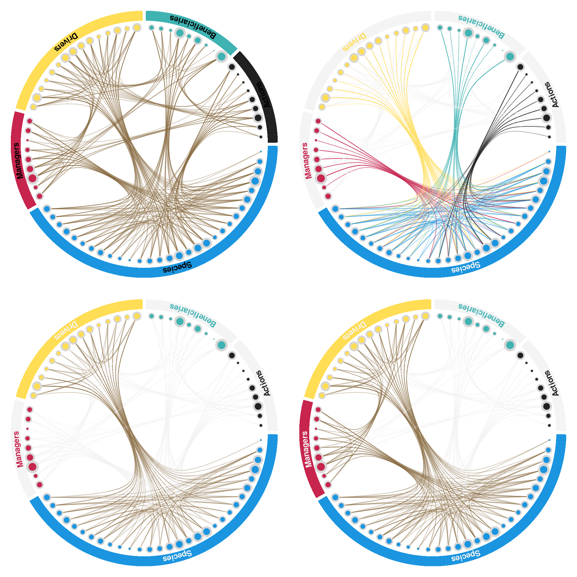
Hierarchical edge bundling using base plot

February 21, 2018

I recently came across a very interesting paper from Laura Dee and collaborators focused on the concept of metanetworks and entitled “Operationalizing Network Theory for Ecosystem Service Assessments” (Dee et al 2017, TREE 32(2):118-130). After reading that article I have begun to revamp the context of my thesis around the concept of metanetworks to include environmental impact assessment and cumulative impacts assessment within such a framework.

Work extensively with networks, you quickly realize that coming up with meaningful and useful visualization can be a bit of a challenge. Thinking about which type of visualization to use for this, the notion of using hierarchical edge bundling became very appealing to capture the complexity of network structure at a glance. While this type of visualization can be close to useless at a fine scale to study individual connections, it can be pretty useful to glean insights as to the overall arrangements of links within networks.

With that in mind, I began going through the material available to make hierarchical edge bundling in R. There is quite a bit of material already available on R, but what I found was always through ggraph and ggplot, which I personally don’t enjoy using all that much (e.g. this). I rather prefer having full control and understanding of what I am doing with my visualizations. So, is here the product of this work to generate the figure I wished to create for my thesis!

Libraries

1
2


library(graphicsutils)
pal_insileco <- gpuPalette("insileco")

Data

Let’s start by simulating data for a metanetwork (i.e. a network composed of multiple networks). To make this as simple as possible, I will simply simulate a dataset composed of hierarchical nodes and another one identifying the links between those nodes.

 1
 2
 3
 4
 5
 6
 7
 8
 9
10
11
12
13
14
15
16
17
18
19
20
21
22
23
24
25
26
27
28
29
30
31
32
33
34
35
36
37
38
39


# Individual network nodes
  opt <- options()
  options(stringsAsFactors = FALSE)
  drivers <- data.frame(network = 'Drivers', name = paste0('driver_',1:15))
  species <- data.frame(network = 'Species', name = paste0('species_',1:30))
  actions <- data.frame(network = 'Actions', name = paste0('action_',1:9))
  managers <- data.frame(network = 'Managers', name = paste0('manager_',1:9))
  beneficiaries <- data.frame(network = 'Beneficiaries', name = paste0('beneficiary_',1:9))

# Nodes dataframe
  nodes <- rbind(drivers, species, actions, managers, beneficiaries)

# Simulate links
  links <- data.frame(from = sample(nodes$name, 300, replace = TRUE),
                      to = sample(nodes$name, 300, replace = TRUE))
  links <- links[!duplicated(links), ]   # Remove duplicates
  links <- links[!links$from == links$to, ] # Remove "cannibalism"

# Combine in a single object
  metanetwork <- vector('list', 0)
  metanetwork$nodes <- nodes
  metanetwork$links <- links

head(nodes)
#R>    network     name
#R>  1 Drivers driver_1
#R>  2 Drivers driver_2
#R>  3 Drivers driver_3
#R>  4 Drivers driver_4
#R>  5 Drivers driver_5
#R>  6 Drivers driver_6
head(links)
#R>             from            to
#R>  1 beneficiary_2    species_22
#R>  2     driver_15     species_4
#R>  3    species_13     driver_12
#R>  4     species_6    species_21
#R>  5    species_19 beneficiary_4
#R>  6     manager_2      action_5

Circle functions

Now that we have the nodes and links, we need to create the necessary functions that will allow us to position our data on a circular graph.

Circle coordinates

The first function we need will be used to generate the x and y coordinates of a circle for a given angle and circle radius, which we can obtain with some circle trigonometry.

 1
 2
 3
 4
 5
 6
 7
 8
 9
10


# Let's begin by creating a function that will give us the x and y coordinates
# of the outside of a circle given a certain radius
coordCircle <- function(theta = NULL, radius = 1) {
  data.frame(x = radius * cos(theta),
             y = radius * sin(theta))
  }

coordCircle(theta = pi, radius = 1)
#R>     x            y
#R>  1 -1 1.224647e-16

Group boundaries

The second function that we need is one that will allow us to distribute groups on the circular plot according to the number of elements composing that group. In essence, we wish to provide the upper and lower boundaries of each individual network composing the metanetwork. We may also want to add a gap between the individual networks on the graph. This will make the visual aspect of the graph more appealing.

 1
 2
 3
 4
 5
 6
 7
 8
 9
10
11
12
13
14
15
16
17
18
19
20
21
22
23
24
25
26
27
28
29


bound <- function(metanetwork, gap = .025, addGap = TRUE) {
  # Metanetwork list composed of "nodes" and "links"
  # Size of gap between groups on the graph
  # addGap logical whether to add gap or not
  nGroup <- as.data.frame(table(metanetwork$nodes$network))
  nGroup$Prop <- nGroup$Freq / sum(nGroup$Freq)
  nGroup$spanDeg <- 2 * pi * nGroup$Prop
  nGroup$upper <- nGroup$lower <- 0
  for(i in 2:nrow(nGroup)) nGroup$lower[i] <- nGroup$lower[i-1] + nGroup$spanDeg[i-1]
  nGroup$upper <- nGroup$lower + nGroup$spanDeg

  if (addGap) {
    nGroup$lower <- nGroup$lower + gap / 2
    nGroup$upper <- nGroup$upper - gap / 2
  }

  nGroup
}

# Add to metanetworks list
  metanetwork$networkGroup <- bound(metanetwork)

metanetwork$networkGroup
#R>             Var1 Freq      Prop   spanDeg     lower     upper
#R>  1       Actions    9 0.1250000 0.7853982 0.0125000 0.7728982
#R>  2 Beneficiaries    9 0.1250000 0.7853982 0.7978982 1.5582963
#R>  3       Drivers   15 0.2083333 1.3089969 1.5832963 2.8672933
#R>  4      Managers    9 0.1250000 0.7853982 2.8922933 3.6526914
#R>  5       Species   30 0.4166667 2.6179939 3.6776914 6.2706853

Nodes coordinates

Now we need to get the coordinates of the edges so that we can position them on the graph. We also need to get coordinates for each network so that we can build an internal, hierarchical structure to the distribution of edges on the graph that can be used to plot links between edges. These should be distributed as the user wish within the circle using different radius values. As with the groups, we can add a gap between the edges at the beginning and end of the group for visual differentiation between the group.

 1
 2
 3
 4
 5
 6
 7
 8
 9
10
11
12
13
14
15
16
17
18
19
20
21
22
23
24
25
26
27
28
29
30
31
32
33
34
35
36
37
38
39
40
41
42
43
44
45
46
47
48
49
50
51
52
53
54
55
56
57


nodePos <- function(metanetwork, edgeRad = 0.975, groupRad = 0.5, gapEdge = 0.1, addGap = TRUE) {
  # Add x and y columns to nodes and networkGroup data
    metanetwork$nodes$y <- metanetwork$nodes$x <- 0
    metanetwork$networkGroup$y <- metanetwork$networkGroup$x <- 0

  # Get coordinates for all networks
    for(i in 1:nrow(metanetwork$networkGroup)) {
      # Distribute points within each network space
      edgeDeg <- seq((metanetwork$networkGroup$lower[i] + (gapEdge/2)),
                       (metanetwork$networkGroup$upper[i] - (gapEdge/2)),
                       length = metanetwork$networkGroup$Freq[i])

      # Get position for each edge
      nodePos <- coordCircle(theta = edgeDeg, radius = edgeRad)

      # Add to nodes data
      metanetwork$nodes$x[metanetwork$nodes$network == metanetwork$networkGroup$Var1[i]] <- nodePos$x
      metanetwork$nodes$y[metanetwork$nodes$network == metanetwork$networkGroup$Var1[i]] <- nodePos$y

      # Distribute network groups in space
      groupDeg <- mean(c(metanetwork$networkGroup$lower[i],metanetwork$networkGroup$upper[i]))

      # Get position for each group
      groupPos <- coordCircle(theta = groupDeg, radius = groupRad)

      # Add to group data
      metanetwork$networkGroup$x[i] <- groupPos$x
      metanetwork$networkGroup$y[i] <- groupPos$y
    }

  metanetwork
}

metanetwork <- nodePos(metanetwork, edgeRad = .875, groupRad = .5)

head(metanetwork$nodes)
#R>    network     name          x         y
#R>  1 Drivers driver_1 -0.0546519 0.8732916
#R>  2 Drivers driver_2 -0.1282239 0.8655539
#R>  3 Drivers driver_3 -0.2008793 0.8516293
#R>  4 Drivers driver_4 -0.2720989 0.8316172
#R>  5 Drivers driver_5 -0.3413735 0.8056607
#R>  6 Drivers driver_6 -0.4082079 0.7739453
head(metanetwork$networkGroup)
#R>             Var1 Freq      Prop   spanDeg     lower     upper          x          y
#R>  1       Actions    9 0.1250000 0.7853982 0.0125000 0.7728982  0.4619398  0.1913417
#R>  2 Beneficiaries    9 0.1250000 0.7853982 0.7978982 1.5582963  0.1913417  0.4619398
#R>  3       Drivers   15 0.2083333 1.3089969 1.5832963 2.8672933 -0.3043807  0.3966767
#R>  4      Managers    9 0.1250000 0.7853982 2.8922933 3.6526914 -0.4957224 -0.0652631
#R>  5       Species   30 0.4166667 2.6179939 3.6776914 6.2706853  0.1294095 -0.4829629

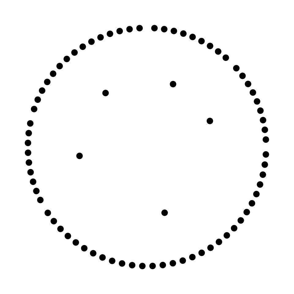
# Visualize the positions of the nodes
# Plot
par(mar = c(0,0,0,0))
plot0()
points(metanetwork$nodes$x, metanetwork$nodes$y, pch = 20, cex = 2)
points(metanetwork$networkGroup$x, metanetwork$networkGroup$y, pch = 20, cex = 2)

Visualization functions

Now we need a few functions to automate the visualization of a few components of the circular plot.

Plot groups

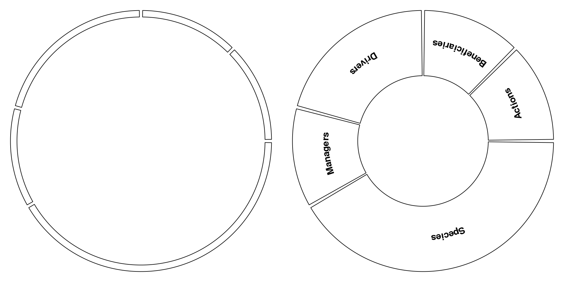
I actually wish to have a box around the edge of my graph identifying each individual network and their name. To do this, we can use the polygon and plotrix::arctext function.

 1
 2
 3
 4
 5
 6
 7
 8
 9
10
11
12
13
14
15
16
17
18
19
20
21
22
23
24
25
26
27
28
29
30
31
32
33
34
35
36
37
38
39
40
41
42
43
44
45
46
47
48
49
50


# We can now use both functions to generate a box for each group on the plot
boxGroup <- function(metanetwork, rad1 = .95, rad2 = 1, colBox = NULL, names = NULL, colNames = NULL, addNames = TRUE, ...) {
  # metanetwork = data list composed of 'nodes', 'links' & 'networkGroup'
  # rad1 = lower boundary for polygons
  # rad2 = upper boundary for polygons
  # colBox = color of boxes
  # names = names of individual networks
  # colNames = color of names
  # addNames = logical, add names of networks to graph
  if (!is.null(colNames) & length(colNames) == 1) {
    colNames <- rep(colNames, nrow(metanetwork$links))
  }

  if (!is.null(colBox) & length(colBox) == 1) {
    colBox <- rep(colBox, nrow(metanetwork$links))
  }

  for(i in 1:nrow(metanetwork$networkGroup)) {
    a <- coordCircle(theta = seq(metanetwork$networkGroup$lower[i],
                             metanetwork$networkGroup$upper[i],
                             length = 200),
                     radius = rad1)

    b <- coordCircle(theta = seq(metanetwork$networkGroup$upper[i],
                             metanetwork$networkGroup$lower[i],
                             length = 200),
                     radius = rad2)

    polygon(rbind(a, b, a[1L,]), col = colBox[i], ...)

    if (addNames) {
      middle <- mean(c(metanetwork$networkGroup$lower[i],
                       metanetwork$networkGroup$upper[i]))
      clockwise <- middle > pi
      plotrix::arctext(x = as.character(metanetwork$networkGroup$Var1[i]),
                       radius = mean(c(rad1,rad2)),
                       middle = middle,
                       col = colNames[i],
                       clockwise = clockwise,
                       font = 2)
    }
  }
}

# Now we can plot
par(mfrow = c(1,2), mar = c(0,0,0,0))
plot0()
boxGroup(metanetwork, addNames = FALSE)
plot0()
boxGroup(metanetwork, rad1 = .5)

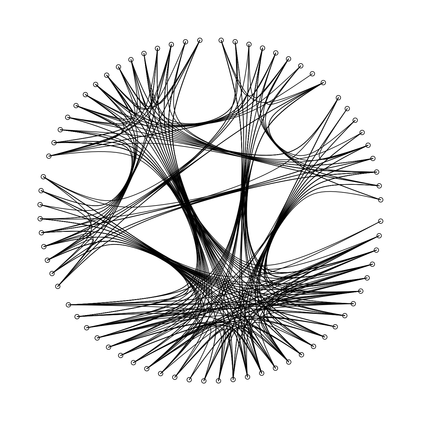
Plot connections

Now we can plot the links between the nodes in our graph using the underlying hierarchical structure identified using the nodePos function created earlier. We can do this using the xspline function.

 1
 2
 3
 4
 5
 6
 7
 8
 9
10
11
12
13
14
15
16
17
18
19
20
21
22
23
24
25
26
27
28
29
30
31


plotLinks <- function(metanetwork, cols = NULL, ...) {
  if (!is.null(cols) & length(cols) == 1) {
    cols <- rep(cols, nrow(metanetwork$links))
  }

  for(i in 1:nrow(metanetwork$links)) {
    link <- metanetwork$links[i,]
    edgeFromID <- which(metanetwork$nodes$name == link$from)
    edgeToID <- which(metanetwork$nodes$name == link$to)
    groupFromID <- which(metanetwork$networkGroup$Var1 == metanetwork$nodes$network[edgeFromID])
    groupToID <- which(metanetwork$networkGroup$Var1 == metanetwork$nodes$network[edgeToID])

    if (metanetwork$nodes$network[edgeFromID] != metanetwork$nodes$network[edgeToID]) {
      linkPath <- rbind(metanetwork$nodes[edgeFromID, c('x','y')],
                        metanetwork$networkGroup[groupFromID, c('x','y')],
                        metanetwork$networkGroup[groupToID, c('x','y')],
                        metanetwork$nodes[edgeToID, c('x','y')])
    } else {
      linkPath <- rbind(metanetwork$nodes[edgeFromID, c('x','y')],
                        metanetwork$networkGroup[groupFromID, c('x','y')],
                        metanetwork$nodes[edgeToID, c('x','y')])
    }

    lines(xspline(linkPath$x, linkPath$y, shape = 1, draw = FALSE), col = cols[i], ...)
  }
}

par(mar = c(0,0,0,0))
plot0()
plotLinks(metanetwork, col = 'black')
points(metanetwork$nodes$x, metanetwork$nodes$y)

Plot metanetwork

1
2
3
4
5
6


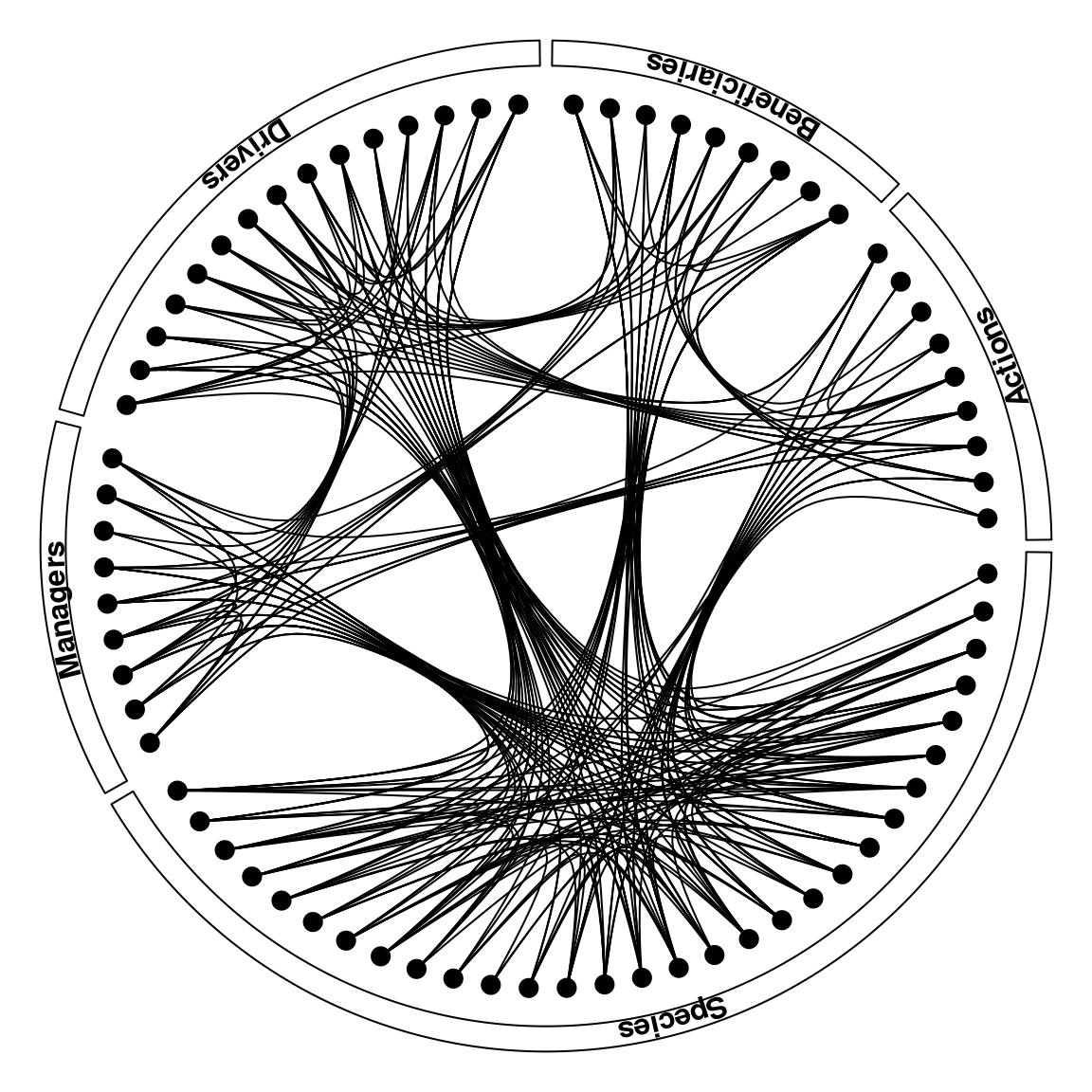
# The plot
par(mar = c(0,0,0,0))
plot0()
boxGroup(metanetwork)
plotLinks(metanetwork, col = 'black')
points(metanetwork$nodes$x, metanetwork$nodes$y, pch = 20, cex = 2)

Customize graph functions

Now we can build functions to customize the graph a little bit, e.g. add colors to links and nodes and change the size of the nodes.

First, let’s give a color to individual networks.

 1
 2
 3
 4
 5
 6
 7
 8
 9
10
11
12
13
14
15
16
17
18
19
20
21
22
23
24
25
26
27
28
29
30


colGroups <- function(metanetwork, colPal = pal_insileco) {
  # Group colors
    metanetwork$networkGroup$cols <- colPal[1:nrow(metanetwork$networkGroup)]

  # Node colors
    metanetwork$nodes$cols <- NA
    for(i in 1:nrow(metanetwork$networkGroup)) {
      metanetwork$nodes$cols[metanetwork$nodes$network == metanetwork$networkGroup$Var1[i]] <- metanetwork$networkGroup$cols[i]
    }

  metanetwork
}

metanetwork <- colGroups(metanetwork, colPal = pal_insileco)

head(metanetwork$nodes)
#R>    network     name          x         y    cols
#R>  1 Drivers driver_1 -0.0546519 0.8732916 #ffdd55
#R>  2 Drivers driver_2 -0.1282239 0.8655539 #ffdd55
#R>  3 Drivers driver_3 -0.2008793 0.8516293 #ffdd55
#R>  4 Drivers driver_4 -0.2720989 0.8316172 #ffdd55
#R>  5 Drivers driver_5 -0.3413735 0.8056607 #ffdd55
#R>  6 Drivers driver_6 -0.4082079 0.7739453 #ffdd55
head(metanetwork$networkGroup)
#R>             Var1 Freq      Prop   spanDeg     lower     upper          x          y    cols
#R>  1       Actions    9 0.1250000 0.7853982 0.0125000 0.7728982  0.4619398  0.1913417 #212121
#R>  2 Beneficiaries    9 0.1250000 0.7853982 0.7978982 1.5582963  0.1913417  0.4619398 #3fb3b2
#R>  3       Drivers   15 0.2083333 1.3089969 1.5832963 2.8672933 -0.3043807  0.3966767 #ffdd55
#R>  4      Managers    9 0.1250000 0.7853982 2.8922933 3.6526914 -0.4957224 -0.0652631 #c7254e
#R>  5       Species   30 0.4166667 2.6179939 3.6776914 6.2706853  0.1294095 -0.4829629 #1b95e0

Second, a function to give a size to nodes based on link frequency.

 1
 2
 3
 4
 5
 6
 7
 8
 9
10
11
12
13
14
15
16
17
18
19
20
21
22
23


# Add size to nodes based on frequency of links to each node
nodeSize <- function(metanetwork, freq = T) {
    if (isTRUE(freq)) {
      nLink <- as.data.frame(table(c(metanetwork$links$from, metanetwork$links$to)), stringsAsFactors = F)
      colnames(nLink)[1L] <- 'name'
      metanetwork$nodes <- dplyr::left_join(metanetwork$nodes, nLink, by = 'name')
      metanetwork$nodes$cex <- (metanetwork$nodes$Freq / max(metanetwork$nodes$Freq))
    } else {
      metanetwork$nodes$cex <- .33
    }

    return(metanetwork)
}

metanetwork <- nodeSize(metanetwork)
head(metanetwork$nodes)
#R>    network     name          x         y    cols Freq    cex
#R>  1 Drivers driver_1 -0.0546519 0.8732916 #ffdd55    7 0.4375
#R>  2 Drivers driver_2 -0.1282239 0.8655539 #ffdd55    7 0.4375
#R>  3 Drivers driver_3 -0.2008793 0.8516293 #ffdd55   12 0.7500
#R>  4 Drivers driver_4 -0.2720989 0.8316172 #ffdd55    6 0.3750
#R>  5 Drivers driver_5 -0.3413735 0.8056607 #ffdd55    6 0.3750
#R>  6 Drivers driver_6 -0.4082079 0.7739453 #ffdd55    7 0.4375

Finally, we can give a color to links or focus on certain individual networks in the metanetwork, or focus on all the links for a single network.

 1
 2
 3
 4
 5
 6
 7
 8
 9
10
11
12
13
14
15
16
17
18
19
20
21
22
23
24
25
26
27
28
29
30
31
32
33
34
35
36
37
38
39
40
41
42
43
44
45
46
47
48
49
50
51
52
53
54
55
56
57
58
59
60
61
62
63
64
65
66
67
68
69
70
71
72
73
74
75
76
77
78
79
80
81
82
83
84
85
86


linkCol <- function(metanetwork, type = 'all', focus = NULL, colLinks = '#876b40', colShadow = '#f4f4f4') {
  # metanetwork = list composed of 'nodes', 'links' and 'networkGroup'
  # type        = type of colors:
  #                 'all' = all links with single color = `colLinks`
  #                 'focus' = focus on the links of identified network
  # focus       = character, name of network(s) to focus on;
  #                 if length(focus) == 1, all links towards a single network
  #                 if length(focus) > 1, links focused on identified networks
  # colLinks    = color of links of `type` == 'all'
  # colShadow   = color of links that we are not focused on

  # Function
  if (type == 'all') {
    metanetwork$links$cols <- colLinks
  }

  if (type == 'focus' & length(focus) == 1) {
    # Box colors
    focusID <- metanetwork$networkGroup$Var1 %in% focus
    colBox <- metanetwork$networkGroup$cols
    metanetwork$networkGroup$cols[!focusID] <- colShadow
    metanetwork$networkGroup$colNames <- colBox
    metanetwork$networkGroup$colNames[focusID] <- colShadow

    # Link colors
    # metanetwork$links$cols <- paste0(colShadow, 88)
    metanetwork$links$cols <- colShadow
    linkCol <- data.frame(from = metanetwork$nodes$network[match(metanetwork$links$from,
                                                                 metanetwork$nodes$name)],
                          to = metanetwork$nodes$network[match(metanetwork$links$to,
                                                                metanetwork$nodes$name)],
                          stringsAsFactors = F)

    linkID <- linkCol$from %in% focus & linkCol$to %in% focus
    metanetwork$links$cols[linkID] <- metanetwork$networkGroup$cols[focusID] # "cannibalism"

    linkID <- (linkCol$from %in% focus | linkCol$to %in% focus) & !linkID
    cols <- paste0(linkCol$from[linkID], linkCol$to[linkID])
    cols <- gsub(focus, '', cols)
    cols <- match(cols, metanetwork$networkGroup$Var1)
    cols <- metanetwork$networkGroup$colNames[cols]
    metanetwork$links$cols[linkID] <- cols
  }

  if (type == 'focus' & length(focus) > 1) {
    # Box colors
    focusID <- metanetwork$networkGroup$Var1 %in% focus
    colBox <- metanetwork$networkGroup$cols
    metanetwork$networkGroup$cols[!focusID] <- colShadow
    metanetwork$networkGroup$colNames <- colBox
    metanetwork$networkGroup$colNames[focusID] <- colShadow

    # Link colors
    metanetwork$links$cols <- colShadow
    linkCol <- data.frame(from = metanetwork$nodes$network[match(metanetwork$links$from,
                                                                 metanetwork$nodes$name)],
                          to = metanetwork$nodes$network[match(metanetwork$links$to,
                                                                metanetwork$nodes$name)],
                          stringsAsFactors = F)

    linkID <- linkCol$from %in% focus & linkCol$to %in% focus
    metanetwork$links$cols[linkID] <- colLinks
  }

  # Add transparency
  metanetwork$links$cols <- paste0(metanetwork$links$cols, '66')

  metanetwork
}

metanetwork <- linkCol(metanetwork, type = 'focus', focus = c('Species','Drivers'))
head(metanetwork$links)
#R>             from            to      cols
#R>  1 beneficiary_2    species_22 #f4f4f466
#R>  2     driver_15     species_4 #876b4066
#R>  3    species_13     driver_12 #876b4066
#R>  4     species_6    species_21 #876b4066
#R>  5    species_19 beneficiary_4 #f4f4f466
#R>  6     manager_2      action_5 #f4f4f466
head(metanetwork$networkGroup)
#R>             Var1 Freq      Prop   spanDeg     lower     upper          x          y    cols colNames
#R>  1       Actions    9 0.1250000 0.7853982 0.0125000 0.7728982  0.4619398  0.1913417 #f4f4f4  #212121
#R>  2 Beneficiaries    9 0.1250000 0.7853982 0.7978982 1.5582963  0.1913417  0.4619398 #f4f4f4  #3fb3b2
#R>  3       Drivers   15 0.2083333 1.3089969 1.5832963 2.8672933 -0.3043807  0.3966767 #ffdd55  #f4f4f4
#R>  4      Managers    9 0.1250000 0.7853982 2.8922933 3.6526914 -0.4957224 -0.0652631 #f4f4f4  #c7254e
#R>  5       Species   30 0.4166667 2.6179939 3.6776914 6.2706853  0.1294095 -0.4829629 #1b95e0  #f4f4f4

Metanetwork function

Now we could wrap all of this in a single function.

 1
 2
 3
 4
 5
 6
 7
 8
 9
10
11
12
13
14
15
16
17
18
19
20
21
22
23
24
25
26
27
28
29
30
31
32
33
34
35
36
37
38
39
40
41
42
43
44
45
46
47
48
49
50
51
52
53
54
55
56
57
58
59
60
61
62
63
64
65
66
67
68
69
70


plotMetanetwork <- function(metanetwork,
                            rad1 = .925,
                            rad2 = 1,
                            sizeEdge = T,
                            colPal = pal_insileco,
                            type = 'all',
                            focus = NULL,
                            colLinks = '#876b40',
                            colShadow = '#f4f4f4',
                            shadowEdge = TRUE
                          ) {

  # Metanetwork = list composed of 'nodes' and 'links'
  # rad1 = lower boundary for individual networks
  # rad2 = upper boundary for individual networks
  # colPal = color palette
  # colLinks = color for links

  # Function
  # Boundaries of individual networks
  metanetwork$networkGroup <- bound(metanetwork)

  # Node coordinates
  metanetwork <- nodePos(metanetwork, edgeRad = .875, groupRad = .5)

  # Colors
  metanetwork <- colGroups(metanetwork, colPal = colPal)

  # Node size
  metanetwork <- nodeSize(metanetwork, freq = sizeEdge)

  # Link col
  metanetwork <- linkCol(metanetwork, type = type, focus = focus, colLinks = colLinks, colShadow = colShadow)

  # Plot
  par(mar = c(0,0,0,0))
  plot0()
  boxGroup(metanetwork,
           rad1 = rad1,
           colBox = metanetwork$networkGroup$cols,
           colNames = metanetwork$networkGroup$colNames,
           border = 'transparent')
  plotLinks(metanetwork,
            col = metanetwork$links$cols)
  if (shadowEdge) {
    points(metanetwork$nodes$x,
           metanetwork$nodes$y,
           pch = 20,
           cex = (metanetwork$nodes$cex * 5),
           col = '#d7d7d7')
  }

  points(metanetwork$nodes$x,
         metanetwork$nodes$y,
         pch = 20,
         cex = (metanetwork$nodes$cex * 3),
         col = metanetwork$nodes$cols)
}

# The data
metanetwork <- vector('list', 0)
metanetwork$nodes <- nodes
metanetwork$links <- links

# The plot
par(mfrow = c(2,2), bg = "transparent")
plotMetanetwork(metanetwork)
plotMetanetwork(metanetwork, type = 'focus', focus = 'Species')
plotMetanetwork(metanetwork, type = 'focus', focus = c('Species', 'Drivers'))
plotMetanetwork(metanetwork, type = 'focus', focus = c('Species', 'Drivers', 'Managers'))

1

opt <- options()

Display information relative to the R session used to render this post.

 1
 2
 3
 4
 5
 6
 7
 8
 9
10
11
12
13
14
15
16
17
18
19
20
21
22
23
24
25
26
27
28
29
30
31
32
33
34
35


sessionInfo()
#R>  R version 4.4.2 (2024-10-31)
#R>  Platform: x86_64-pc-linux-gnu
#R>  Running under: Ubuntu 22.04.5 LTS
#R>  
#R>  Matrix products: default
#R>  BLAS:   /usr/lib/x86_64-linux-gnu/openblas-pthread/libblas.so.3 
#R>  LAPACK: /usr/lib/x86_64-linux-gnu/openblas-pthread/libopenblasp-r0.3.20.so;  LAPACK version 3.10.0
#R>  
#R>  locale:
#R>   [1] LC_CTYPE=C.UTF-8       LC_NUMERIC=C           LC_TIME=C.UTF-8        LC_COLLATE=C.UTF-8    
#R>   [5] LC_MONETARY=C.UTF-8    LC_MESSAGES=C.UTF-8    LC_PAPER=C.UTF-8       LC_NAME=C             
#R>   [9] LC_ADDRESS=C           LC_TELEPHONE=C         LC_MEASUREMENT=C.UTF-8 LC_IDENTIFICATION=C   
#R>  
#R>  time zone: UTC
#R>  tzcode source: system (glibc)
#R>  
#R>  attached base packages:
#R>  [1] stats     graphics  grDevices utils     datasets  methods   base     
#R>  
#R>  other attached packages:
#R>  [1] graphicsutils_1.6.0.9000 inSilecoRef_0.1.1       
#R>  
#R>  loaded via a namespace (and not attached):
#R>   [1] sass_0.4.9        utf8_1.2.4        generics_0.1.3    xml2_1.3.6        blogdown_1.19    
#R>   [6] stringi_1.8.4     httpcode_0.3.0    digest_0.6.37     magrittr_2.0.3    evaluate_1.0.1   
#R>  [11] bookdown_0.41     fastmap_1.2.0     plyr_1.8.9        jsonlite_1.8.9    backports_1.5.0  
#R>  [16] crul_1.5.0        promises_1.3.0    fansi_1.0.6       jquerylib_0.1.4   bibtex_0.5.1     
#R>  [21] cli_3.6.3         shiny_1.9.1       rlang_1.1.4       plotrix_3.8-4     cachem_1.1.0     
#R>  [26] yaml_2.3.10       tools_4.4.2       dplyr_1.1.4       httpuv_1.6.15     DT_0.33          
#R>  [31] rcrossref_1.2.0   curl_6.0.0        vctrs_0.6.5       R6_2.5.1          mime_0.12        
#R>  [36] lifecycle_1.0.4   stringr_1.5.1     fs_1.6.5          htmlwidgets_1.6.4 miniUI_0.1.1.1   
#R>  [41] pkgconfig_2.0.3   bslib_0.8.0       pillar_1.9.0      later_1.3.2       glue_1.8.0       
#R>  [46] Rcpp_1.0.13-1     xfun_0.49         tibble_3.2.1      tidyselect_1.2.1  knitr_1.49       
#R>  [51] xtable_1.8-4      htmltools_0.5.8.1 rmarkdown_2.29    compiler_4.4.2