Vector Fields.

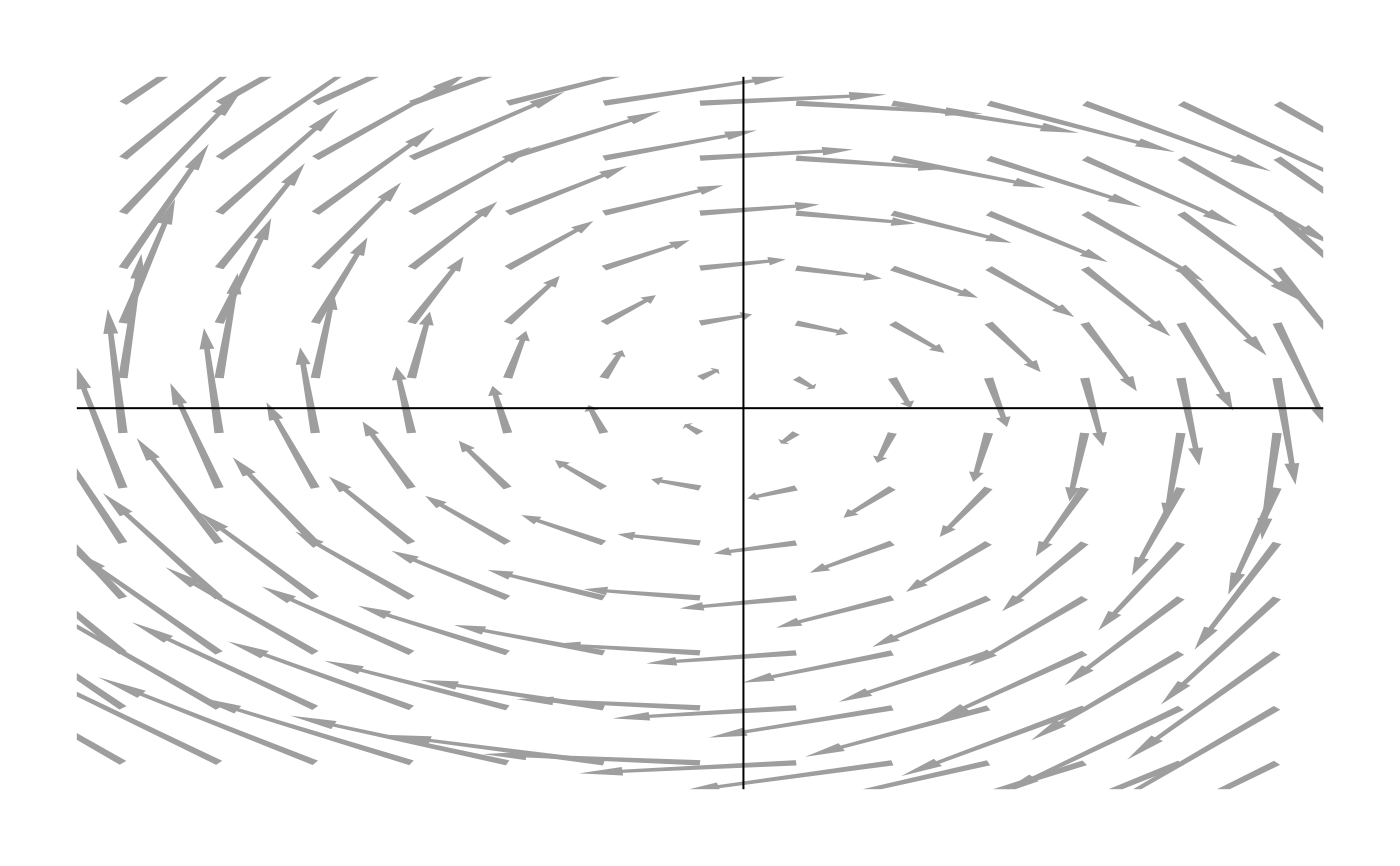
Draw a vector field associated to a system of at least two ODE.

vecfield2d(
  coords,
  FUN,
  args = NULL,
  ndim = NULL,
  slices = c(1, 2),
  fixed = NULL,
  cex.x = 0.25,
  cex.y = cex.x,
  log = FALSE,
  add = FALSE,
  ...
)

Arguments

coords	a matrix with two columns or more that is optionally used to alternatively define the coordinates of the vector field.
FUN	the function that describes the dynamical system (see details).
args	the parameters of the dynamical system (see details).
ndim	number of dimension of the system. If NULL the values is based on coords and slice
slices	a vector of 2 elements providing the dimensions to be displayed, (default set to c(1,2)).
fixed	the values used for non drawn dimension, if NULL the values will be set to 0.
cex.x	the magnification coefficient to be used for lengths of vectors along the x axis.
cex.y	the magnification coefficient to be used for lengths of vectors along the y axis.
log	a logical. If TRUE, the lengths of arrows are log-transformed.
add	a logical. If TRUE, the vector field is added on the current plot.
...	additional arguments to be passed to arrows().

Details

The FUN function must be a function of at least two arguments. The first argument must contain the dynamical variables as a vector and the second arguments must contain all the other parameters that shapes the dynamical system. When some dimensions are missing, the order of fixed is the one in FUN once the drawn dimension are withdrawn.

Examples

systLin <- function(X, beta){
    Y <- matrix(0,ncol=2)
    Y[1L] <- beta[1,1]*X[1L]+beta[1,2]*X[2L]
    Y[2L] <- beta[2,1]*X[1L]+beta[2,2]*X[2L]
    return(Y)
}
seqx <- seq(-2,2,0.31)
seqy <- seq(-2,2,0.31)
beta1 <- matrix(c(0,-1,1,0),2)
# Plot 1:
vecfield2d(coords=expand.grid(seqx, seqy), FUN=systLin, args=list(beta=beta1))
# Plot 2:
graphics::par(mar=c(2,2,2,2))
vecfield2d(coords=expand.grid(seqx, seqy), FUN=systLin,
   args=list(beta=beta1), cex.x=0.35, cex.arr=0.25,
   border=NA,cex.hh=1, cex.shr=0.6, col=8)
graphics::abline(v=0,h=0)