class: title-slide, middle # Touchdown your research with <img src="assets/img/rmarkdown.png" style="vertical-align: middle;margin:10px" width="120px"></img> .instructors[ **QCBS R Workshop** Steve Vissault, Marie-Hélène Brice, David Beauchesne & Kevin Cazelles ] <a href="https://insileco.github.io"><img src="assets/img/inSileco.png" width="80px"></img></a> <div style="color:white;"> .font60[Adapted from [Alison Hill](https://rmd4medicine.netlify.com/slides/01-rmd-anatomy.html#8)] </div> --- # Workshop setup - Make sure you have an updated version of [RStudio](https://rstudio.com/products/rstudio/download/) - Install the [code version-control system Git](https://git-scm.com/downloads) - Create a [Github account](https://github.com/join?source=header-home) - Run the following R command: ```r install.packages(c("rmarkdown", "htmlwidgets", "bookdown", "blogdown", "DT", "leaflet", "rbokeh")) ``` - Be prepared to turn into a geek or just learn cool stuff --- class: clear, middle, center <img src="assets/img/rmarkdown_rockstar.png" width="80%" /> .font80[Illustration from [@allisonhorst](https://twitter.com/allison_horst)] --- class: clear, middle ## R Markdown universe R Markdown produces dynamic document in a variety of format. ### Opens new possibilities with R: * make CV, poster & online presentation * format scientific paper (`rticles`) * help to document your research through notebook (`bookdown`) * build an academic blog or website (`blogdown`) --- class: clear, middle ## But what's R Markdown? - ["An authoring framework for data science."](https://rmarkdown.rstudio.com/lesson-1.html) (✔️) - [A document format (.Rmd).](https://bookdown.org/yihui/rmarkdown/) (✔️) - [An R package named rmarkdown.](https://rmarkdown.rstudio.com/docs/) (✔️) - ["A tool for integrating text, code, and results."](https://r4ds.had.co.nz/communicate-intro.html) (✔️) - ["A file format for making dynamic documents with R."](https://rmarkdown.rstudio.com/articles_intro.html) (✔️) - ["A computational document."](http://radar.oreilly.com/2011/07/wolframs-computational-documen.html) (✔️) - [Wizardry.](https://raw.githubusercontent.com/allisonhorst/stats-illustrations/master/rstats-artwork/rmarkdown_wizards.png) (🧙) --- class: inverse, center, middle # Workshop objective <html><div style='float:left'></div><hr color='#ffdd55' style="margin-top:-60px" size=1px width=720px></html> ## Build a website | notebook | presentation with <code style="color:rgb(11, 43, 70)">rmarkdown</code> and deploys it on the web --- class: inverse, center, middle # Basic Anatomy <html><div style='float:left'></div><hr color='#ffdd55' style="margin-top: -60px;" size=1px width=720px></html> ## R Markdown (<i class="ion ion-social-markdown "></i> + <i class="fab fa-r-project "></i>) --- # <i class="fas fa-gamepad "></i> Exercice 1. Open RStudio 2. File > New File > R Markdown 3. Fill the fields *author* and *title* 4. Set default output format to HTML 5. Look at the source, then 🧶 Knit to HTML. ### Try to identify these parts in the source and the output: - The metadata - The text <i class="ion ion-social-markdown "></i> - The code <i class="fab fa-r-project "></i> - The output <div class="countdown" id="timer_5da1c55e" style="right:0;bottom:0;" data-warnwhen="0"> <code class="countdown-time"><span class="countdown-digits minutes">03</span><span class="countdown-digits colon">:</span><span class="countdown-digits seconds">00</span></code> </div> --- # How does R Markdown work? .pull-left[ <img src="assets/img/Rmdformat.png" width="100%" /> ] .pull-right[ - 🤷 - I press knit, a document appears, and I believe that anything happening in between could be actual magic. - `knitr` executes the code and converts `.Rmd` to `.md`; Pandoc renders the `.md` file to the output format you want. ] --- class: middle, center, clear 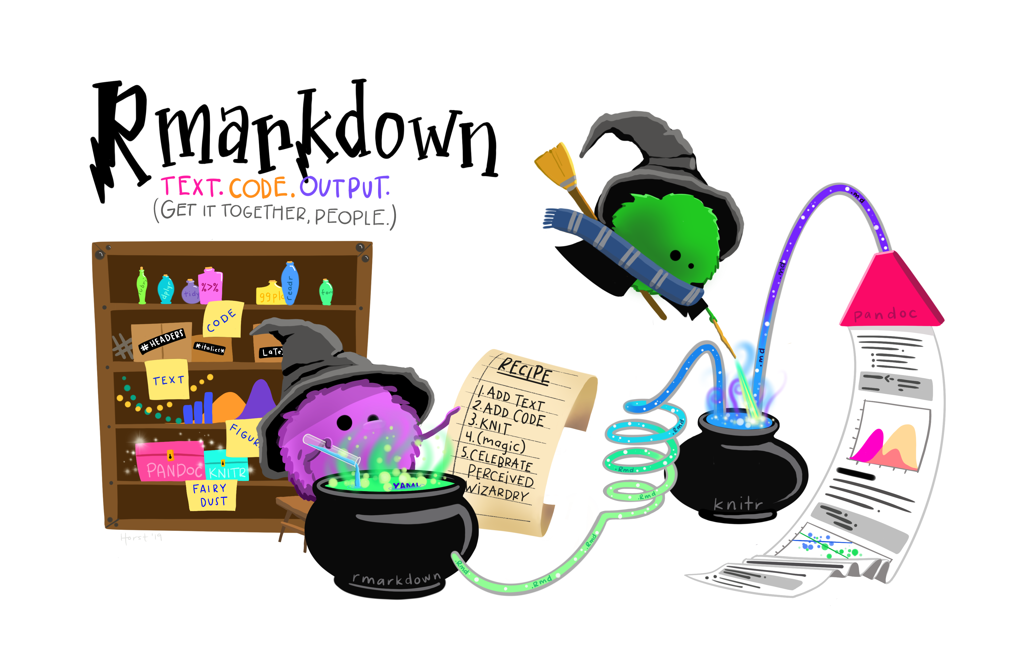 .font80[Illustration from [@allisonhorst](https://twitter.com/allison_horst)] --- class: inverse, center, middle # Document metadata <html><div style='float:left'></div><hr color='#ffdd55' style="margin-top: -60px;" size=1px width=720px></html> ## R Markdown (<i class="ion ion-social-markdown "></i> + <i class="fab fa-r-project "></i>) --- # Metadata and options Metadata with options are defined in the header of the `.Rmd` document as a set of `key` and `value` (YAML syntax). .pull-left[ ### One output ```r --- output: html_document --- ``` ] .pull-right[ ### Two outputs ```r --- output: html_document: toc: true pdf_document: toc: false --- ``` ] Options available depend on the output. See `?html_document `, `?pdf_document`, `?word_document` ??? - You have already notice the keys `author`, `title`, `date` - What's the purpose of the indentation? --- # <i class="fas fa-gamepad "></i> Exercice ### Edit the output options Use `?html_document` from your R console to: 1. Add a floating table of contents 2. Add a theme 3. Use the "kable" method to print data frames 🧶 Knit to HTML to see the output. If this was easy, try to embed the Rmd source code to download. <div class="countdown" id="timer_5da1c4c0" style="right:0;bottom:0;" data-warnwhen="0"> <code class="countdown-time"><span class="countdown-digits minutes">03</span><span class="countdown-digits colon">:</span><span class="countdown-digits seconds">00</span></code> </div> ??? ### Answer ```r --- output: html_document: toc: true toc_float: true theme: flatly df_print: kable code_download: true --- We have done a brief overview of the document options (the shape), we now make an introduction of the content ``` --- class: inverse, center, middle # Document content <html><div style='float:left'></div><hr color='#ffdd55' style="margin-top: -60px;" size=1px width=720px></html> ## R Markdown (<i class="ion ion-social-markdown "></i> + <i class="fab fa-r-project "></i>) --- class: clear, middle, center <img src="assets/img/rmarkdown_rockstar.png" width="80%" /> .font80[Illustration from [@allisonhorst](https://twitter.com/allison_horst)] --- class: inverse, center, middle # Text formatting <html><div style='float:left'></div><hr color='#ffdd55' style="margin-top: -60px;" size=1px width=720px></html> ## Markdown <i class="ion ion-social-markdown "></i> --- # Text style .pull-left[ ````md # Header 1 ## Header 2 ### Header 3 #### Header 4 *italic* or _italic_ **bold** `code` ```r library(tibble) data(iris) glimpse(as_tibble(iris)) ``` ```` ] .pull-right[ <h1 style="margin:0px;padding:0px">Header 1</h1> <h2 style="margin:0px;padding:0px">Header 2</h2> <h3 style="margin:0px;padding:0px">Header 3</h3> <h4 style="margin:0px;padding:0px">Header 4</h4> *italic* or _italic_ **bold** `code` ```r library(tibble) data(iris) glimpse(as_tibble(iris)) ``` ] ??? Headers help you to structure your Rmd Document --- # Lists .pull-left[ ```md Lorem ipsum dolor sit amet, consectetur adipiscing elit. - Cras convallis purus. - Nunc faucibus. - Maecenas ipsum dolor. Nulla vehicula metus vel tortor venenatis luctus. Etiam tempus sit amet ligula nec pretium. Aenean ultrices massa sed pulvinar pulvinar. 1. Duis aliquam commodo volutpat. 1. Mauris ultrices. 1. Aliquam eu erat. ``` ] .pull-right[ Lorem ipsum dolor sit amet, consectetur adipiscing elit. * Cras convallis purus. - Nunc faucibus. * Maecenas ipsum dolor. Nulla vehicula metus vel tortor venenatis luctus. 1. Duis aliquam commodo volutpat. 1. Mauris ultrices. 1. Aliquam eu erat. ] --- # Images .pull-left[ ```md  ``` ] .pull-right[  ] --- # Links .pull-left[ ```md [Hulk vs Trump](https://media.giphy.com/media/MkGyW2cOH7uhO/giphy.gif)  ``` ] .pull-right[ [Hulk vs Trump](https://media.giphy.com/media/MkGyW2cOH7uhO/giphy.gif)  ] --- # Tables .pull-left[ ### Syntax ```md | Time | Session | Topic | |:--------------|:-------:|---------:| | _left_ | _center_| _right_ | | 01:00 - 01:50 | 1 | Anatomy | | 01:50 - 02:00 | | *Break* | | 02:00 - 02:45 | 2 | Tables | | 02:45 - 03:00 | | *Break* | ``` ] .pull-right[ ### Output | Time | Session | Topic | |:--------------|:-------:|---------:| | _left_ | _center_| _right_ | | 01:00 - 01:50 | 1 | Anatomy | | 01:50 - 02:00 | | *Break* | | 02:00 - 02:45 | 2 | Tables | | 02:45 - 03:00 | | *Break* | ] - <i class="fas fa-exclamation-triangle "></i> the `:` specify the alignement. - Not convenient for long table, we will use instead <i class="fab fa-r-project "></i> to print the markdown table for us. --- class: inverse, center, middle # Code chunks <html><div style='float:left'></div><hr color='#ffdd55'style="margin-top: -60px;" size=1px width=720px></html> ## The <i class="fab fa-r-project "></i> part --- # Chunks ````md This text is written in markdown ```{r} library(tibble) data(iris) head(iris) ``` ```` - <i class="fas fa-exclamation-triangle "></i> `r` between brackets `{}`, why is that? - Where is the <i class="fab fa-r-project "></i> code and the <i class="ion ion-social-markdown "></i> section? --- # Chunks ### Code ```r library(tibble) data(iris) head(iris) ``` ### Print output ``` ## Sepal.Length Sepal.Width Petal.Length Petal.Width Species ## 1 5.1 3.5 1.4 0.2 setosa ## 2 4.9 3.0 1.4 0.2 setosa ## 3 4.7 3.2 1.3 0.2 setosa ## 4 4.6 3.1 1.5 0.2 setosa ## 5 5.0 3.6 1.4 0.2 setosa ## 6 5.4 3.9 1.7 0.4 setosa ``` --- # Chunks .pull-left[ ### Code ```r library(ggplot2) data(iris) ggplot( data=iris, aes(x = Sepal.Length, y = Sepal.Width) ) + geom_point( aes(color=Species, shape=Species) ) + xlab("Sepal Length") + ylab("Sepal Width") + ggtitle("Sepal Length-Width") ``` ] .pull-right[ ### Graphic output 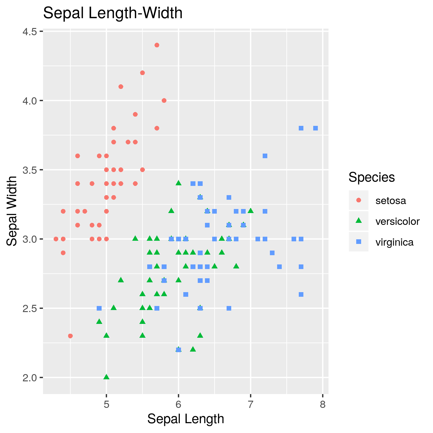<!-- --> ] --- # Chunks .pull-left[ ### Code ```r library(leaflet) leaflet(height=400, width=400) %>% addTiles() %>% addMarkers(lng=174.768, lat=-36.852, popup="The birthplace of R") ``` ] .pull-right[ <h3 style="margin-bottom:10px;">Map</h3> <div id="htmlwidget-d9cef98fe54d70eacf2d" style="width:400px;height:400px;" class="leaflet html-widget"></div> <script type="application/json" data-for="htmlwidget-d9cef98fe54d70eacf2d">{"x":{"options":{"crs":{"crsClass":"L.CRS.EPSG3857","code":null,"proj4def":null,"projectedBounds":null,"options":{}}},"calls":[{"method":"addTiles","args":["//{s}.tile.openstreetmap.org/{z}/{x}/{y}.png",null,null,{"minZoom":0,"maxZoom":18,"tileSize":256,"subdomains":"abc","errorTileUrl":"","tms":false,"noWrap":false,"zoomOffset":0,"zoomReverse":false,"opacity":1,"zIndex":1,"detectRetina":false,"attribution":"© <a href=\"http://openstreetmap.org\">OpenStreetMap<\/a> contributors, <a href=\"http://creativecommons.org/licenses/by-sa/2.0/\">CC-BY-SA<\/a>"}]},{"method":"addMarkers","args":[-36.852,174.768,null,null,null,{"interactive":true,"draggable":false,"keyboard":true,"title":"","alt":"","zIndexOffset":0,"opacity":1,"riseOnHover":false,"riseOffset":250},"The birthplace of R",null,null,null,null,{"interactive":false,"permanent":false,"direction":"auto","opacity":1,"offset":[0,0],"textsize":"10px","textOnly":false,"className":"","sticky":true},null]}],"limits":{"lat":[-36.852,-36.852],"lng":[174.768,174.768]}},"evals":[],"jsHooks":[]}</script> ] --- # Chunks .pull-left[ ### Code ```r library(rbokeh) p <- figure() %>% ly_points(Sepal.Length, Sepal.Width, data = iris, color = Species, glyph = Species, hover = list(Sepal.Length, Sepal.Width)) p ``` ] .pull-right[ <h3 style="margin-bottom:10px;">Map</h3> <div id="htmlwidget-1d4d0ec371fa6b9d6add" style="width:400px;height:400px;" class="rbokeh html-widget"></div> <script type="application/json" data-for="htmlwidget-1d4d0ec371fa6b9d6add">{"x":{"elementid":"93549cba0a787421afc66318ae550ca6","modeltype":"Plot","modelid":"8d823230c9142afec509818bd39b2c1a","docid":"47537f30831bdcd1f54c8983b783281a","docs_json":{"47537f30831bdcd1f54c8983b783281a":{"version":"0.12.2","title":"Bokeh Figure","roots":{"root_ids":["8d823230c9142afec509818bd39b2c1a"],"references":[{"type":"Plot","id":"8d823230c9142afec509818bd39b2c1a","attributes":{"id":"8d823230c9142afec509818bd39b2c1a","plot_width":400,"plot_height":400,"sizing_mode":"scale_both","x_range":{"type":"Range1d","id":"8cf3f0b18ad4b252d6bbb07d627da697"},"y_range":{"type":"Range1d","id":"b597ea17d5a97c6b8e25575cd5a21c72"},"left":[{"type":"LinearAxis","id":"8b1b4e7195f80b1b766d25136cb49525"}],"below":[{"type":"LinearAxis","id":"2d745b3b87be688d5364e7caad2df8d0"}],"right":[],"above":[],"renderers":[{"type":"BoxAnnotation","id":"61f2ab10c458157a1a358c14c91ffb31"},{"type":"GlyphRenderer","id":"e2c7003967dce2633344392e91df1e6c"},{"type":"GlyphRenderer","id":"5296b1a207e1f7416585f9108e1ee805"},{"type":"GlyphRenderer","id":"b5c300402119ebe3c2ed05375406d610"},{"type":"GlyphRenderer","id":"f366dea0678386e04cfaad4ea0a007dd"},{"type":"GlyphRenderer","id":"ea2b662d230a7e0be95135494cd3000c"},{"type":"GlyphRenderer","id":"c27224bda781f853ef03f817d5fbfb99"},{"type":"Legend","id":"d521d8fcc9a14366b7faeb756c65ec3b"},{"type":"LinearAxis","id":"2d745b3b87be688d5364e7caad2df8d0"},{"type":"Grid","id":"847fc0b36165c41c2b845055d6fdf656"},{"type":"LinearAxis","id":"8b1b4e7195f80b1b766d25136cb49525"},{"type":"Grid","id":"a0450587d813e311e246bae48234f5e7"}],"extra_y_ranges":{},"extra_x_ranges":{},"tags":[],"min_border_left":4,"min_border_right":4,"min_border_top":4,"min_border_bottom":4,"lod_threshold":null,"toolbar":{"type":"Toolbar","id":"e71a331a2b5ac72756a0488165d99830"},"tool_events":{"type":"ToolEvents","id":"d055ee8dfa2036865545fad2e8207146"}},"subtype":"Figure"},{"type":"Toolbar","id":"e71a331a2b5ac72756a0488165d99830","attributes":{"id":"e71a331a2b5ac72756a0488165d99830","tags":[],"active_drag":"auto","active_scroll":"auto","active_tap":"auto","tools":[{"type":"PanTool","id":"c145b2ec4dfd3c39a05468601a3d71a9"},{"type":"WheelZoomTool","id":"8bbfc4db105dd4cd7e1013a70c5bfeee"},{"type":"BoxZoomTool","id":"26270b129602ba1da9568b868a5907c0"},{"type":"ResetTool","id":"d1c878754e89ed61f37e411d75480800"},{"type":"SaveTool","id":"932623ac4cd08f437c56791aeb40a486"},{"type":"HelpTool","id":"376826e7cb28fae2c1730ae46855903e"},{"type":"HoverTool","id":"f8c8d95f0132943661aaa4977856cb38"},{"type":"HoverTool","id":"28262706f4d737fb99f85634118a24b6"},{"type":"HoverTool","id":"92df848058bb89eaaf4a9dd837883198"}],"logo":null}},{"type":"PanTool","id":"c145b2ec4dfd3c39a05468601a3d71a9","attributes":{"id":"c145b2ec4dfd3c39a05468601a3d71a9","tags":[],"plot":{"type":"Plot","id":"8d823230c9142afec509818bd39b2c1a","subtype":"Figure"},"dimensions":["width","height"]}},{"type":"ToolEvents","id":"d055ee8dfa2036865545fad2e8207146","attributes":{"id":"d055ee8dfa2036865545fad2e8207146","tags":[]},"geometries":[]},{"type":"WheelZoomTool","id":"8bbfc4db105dd4cd7e1013a70c5bfeee","attributes":{"id":"8bbfc4db105dd4cd7e1013a70c5bfeee","tags":[],"plot":{"type":"Plot","id":"8d823230c9142afec509818bd39b2c1a","subtype":"Figure"},"dimensions":["width","height"]}},{"type":"BoxAnnotation","id":"61f2ab10c458157a1a358c14c91ffb31","attributes":{"id":"61f2ab10c458157a1a358c14c91ffb31","tags":[],"line_color":{"units":"data","value":"black"},"line_alpha":{"units":"data","value":1},"fill_color":{"units":"data","value":"lightgrey"},"fill_alpha":{"units":"data","value":0.5},"line_dash":[4,4],"line_width":{"units":"data","value":2},"level":"overlay","top_units":"screen","bottom_units":"screen","left_units":"screen","right_units":"screen","render_mode":"css"}},{"type":"BoxZoomTool","id":"26270b129602ba1da9568b868a5907c0","attributes":{"id":"26270b129602ba1da9568b868a5907c0","tags":[],"plot":{"type":"Plot","id":"8d823230c9142afec509818bd39b2c1a","subtype":"Figure"},"overlay":{"type":"BoxAnnotation","id":"61f2ab10c458157a1a358c14c91ffb31"}}},{"type":"ResetTool","id":"d1c878754e89ed61f37e411d75480800","attributes":{"id":"d1c878754e89ed61f37e411d75480800","tags":[],"plot":{"type":"Plot","id":"8d823230c9142afec509818bd39b2c1a","subtype":"Figure"}}},{"type":"SaveTool","id":"932623ac4cd08f437c56791aeb40a486","attributes":{"id":"932623ac4cd08f437c56791aeb40a486","tags":[],"plot":{"type":"Plot","id":"8d823230c9142afec509818bd39b2c1a","subtype":"Figure"}}},{"type":"HelpTool","id":"376826e7cb28fae2c1730ae46855903e","attributes":{"id":"376826e7cb28fae2c1730ae46855903e","tags":[],"plot":{"type":"Plot","id":"8d823230c9142afec509818bd39b2c1a","subtype":"Figure"},"redirect":"http://hafen.github.io/rbokeh","help_tooltip":"Click to learn more about rbokeh."}},{"type":"HoverTool","id":"f8c8d95f0132943661aaa4977856cb38","attributes":{"id":"f8c8d95f0132943661aaa4977856cb38","tags":[],"plot":{"type":"Plot","id":"8d823230c9142afec509818bd39b2c1a","subtype":"Figure"},"renderers":[{"type":"GlyphRenderer","id":"e2c7003967dce2633344392e91df1e6c"}],"names":[],"anchor":"center","attachment":"horizontal","line_policy":"prev","mode":"mouse","point_policy":"snap_to_data","tooltips":[["Sepal.Length","@hover_col_1"],["Sepal.Width","@hover_col_2"]]}},{"type":"ColumnDataSource","id":"d4acd6f956e70c93a7fcf723cb68d29c","attributes":{"id":"d4acd6f956e70c93a7fcf723cb68d29c","tags":[],"column_names":["x","y","line_color","fill_color","hover_col_1","hover_col_2"],"selected":[],"data":{"x":[5.1,4.9,4.7,4.6,5,5.4,4.6,5,4.4,4.9,5.4,4.8,4.8,4.3,5.8,5.7,5.4,5.1,5.7,5.1,5.4,5.1,4.6,5.1,4.8,5,5,5.2,5.2,4.7,4.8,5.4,5.2,5.5,4.9,5,5.5,4.9,4.4,5.1,5,4.5,4.4,5,5.1,4.8,5.1,4.6,5.3,5],"y":[3.5,3,3.2,3.1,3.6,3.9,3.4,3.4,2.9,3.1,3.7,3.4,3,3,4,4.4,3.9,3.5,3.8,3.8,3.4,3.7,3.6,3.3,3.4,3,3.4,3.5,3.4,3.2,3.1,3.4,4.1,4.2,3.1,3.2,3.5,3.6,3,3.4,3.5,2.3,3.2,3.5,3.8,3,3.8,3.2,3.7,3.3],"line_color":["#1F77B4","#1F77B4","#1F77B4","#1F77B4","#1F77B4","#1F77B4","#1F77B4","#1F77B4","#1F77B4","#1F77B4","#1F77B4","#1F77B4","#1F77B4","#1F77B4","#1F77B4","#1F77B4","#1F77B4","#1F77B4","#1F77B4","#1F77B4","#1F77B4","#1F77B4","#1F77B4","#1F77B4","#1F77B4","#1F77B4","#1F77B4","#1F77B4","#1F77B4","#1F77B4","#1F77B4","#1F77B4","#1F77B4","#1F77B4","#1F77B4","#1F77B4","#1F77B4","#1F77B4","#1F77B4","#1F77B4","#1F77B4","#1F77B4","#1F77B4","#1F77B4","#1F77B4","#1F77B4","#1F77B4","#1F77B4","#1F77B4","#1F77B4"],"fill_color":["#1F77B4","#1F77B4","#1F77B4","#1F77B4","#1F77B4","#1F77B4","#1F77B4","#1F77B4","#1F77B4","#1F77B4","#1F77B4","#1F77B4","#1F77B4","#1F77B4","#1F77B4","#1F77B4","#1F77B4","#1F77B4","#1F77B4","#1F77B4","#1F77B4","#1F77B4","#1F77B4","#1F77B4","#1F77B4","#1F77B4","#1F77B4","#1F77B4","#1F77B4","#1F77B4","#1F77B4","#1F77B4","#1F77B4","#1F77B4","#1F77B4","#1F77B4","#1F77B4","#1F77B4","#1F77B4","#1F77B4","#1F77B4","#1F77B4","#1F77B4","#1F77B4","#1F77B4","#1F77B4","#1F77B4","#1F77B4","#1F77B4","#1F77B4"],"hover_col_1":["5.1","4.9","4.7","4.6","5.0","5.4","4.6","5.0","4.4","4.9","5.4","4.8","4.8","4.3","5.8","5.7","5.4","5.1","5.7","5.1","5.4","5.1","4.6","5.1","4.8","5.0","5.0","5.2","5.2","4.7","4.8","5.4","5.2","5.5","4.9","5.0","5.5","4.9","4.4","5.1","5.0","4.5","4.4","5.0","5.1","4.8","5.1","4.6","5.3","5.0"],"hover_col_2":["3.5","3.0","3.2","3.1","3.6","3.9","3.4","3.4","2.9","3.1","3.7","3.4","3.0","3.0","4.0","4.4","3.9","3.5","3.8","3.8","3.4","3.7","3.6","3.3","3.4","3.0","3.4","3.5","3.4","3.2","3.1","3.4","4.1","4.2","3.1","3.2","3.5","3.6","3.0","3.4","3.5","2.3","3.2","3.5","3.8","3.0","3.8","3.2","3.7","3.3"]}}},{"type":"Circle","id":"aaf0180769577575c8be97371d26c5fb","attributes":{"id":"aaf0180769577575c8be97371d26c5fb","tags":[],"size":{"units":"screen","value":10},"visible":true,"line_alpha":{"units":"data","value":1},"fill_alpha":{"units":"data","value":0.5},"x":{"units":"data","field":"x"},"y":{"units":"data","field":"y"},"line_color":{"units":"data","field":"line_color"},"fill_color":{"units":"data","field":"fill_color"}}},{"type":"Circle","id":"90b26fbf51d71798d003cdcf4159f8db","attributes":{"id":"90b26fbf51d71798d003cdcf4159f8db","tags":[],"size":{"units":"screen","value":10},"visible":true,"line_alpha":{"units":"data","value":1},"fill_alpha":{"units":"data","value":0.5},"x":{"units":"data","field":"x"},"y":{"units":"data","field":"y"},"line_color":{"units":"data","value":"#e1e1e1"},"fill_color":{"units":"data","value":"#e1e1e1"}}},{"type":"Circle","id":"0c85cb19c21e3c80daea223a99e2fb35","attributes":{"id":"0c85cb19c21e3c80daea223a99e2fb35","tags":[],"size":{"units":"screen","value":10},"visible":true,"line_alpha":{"units":"data","value":1},"fill_alpha":{"units":"data","value":1},"x":{"units":"data","field":"x"},"y":{"units":"data","field":"y"},"line_color":{"units":"data","field":"line_color"},"fill_color":{"units":"data","field":"fill_color"}}},{"type":"GlyphRenderer","id":"e2c7003967dce2633344392e91df1e6c","attributes":{"id":"e2c7003967dce2633344392e91df1e6c","tags":[],"selection_glyph":null,"nonselection_glyph":{"type":"Circle","id":"90b26fbf51d71798d003cdcf4159f8db"},"hover_glyph":{"type":"Circle","id":"0c85cb19c21e3c80daea223a99e2fb35"},"name":null,"data_source":{"type":"ColumnDataSource","id":"d4acd6f956e70c93a7fcf723cb68d29c"},"glyph":{"type":"Circle","id":"aaf0180769577575c8be97371d26c5fb"}}},{"type":"HoverTool","id":"28262706f4d737fb99f85634118a24b6","attributes":{"id":"28262706f4d737fb99f85634118a24b6","tags":[],"plot":{"type":"Plot","id":"8d823230c9142afec509818bd39b2c1a","subtype":"Figure"},"renderers":[{"type":"GlyphRenderer","id":"5296b1a207e1f7416585f9108e1ee805"}],"names":[],"anchor":"center","attachment":"horizontal","line_policy":"prev","mode":"mouse","point_policy":"snap_to_data","tooltips":[["Sepal.Length","@hover_col_1"],["Sepal.Width","@hover_col_2"]]}},{"type":"ColumnDataSource","id":"8bbae23206058d175c461e60d549be37","attributes":{"id":"8bbae23206058d175c461e60d549be37","tags":[],"column_names":["x","y","line_color","fill_color","hover_col_1","hover_col_2"],"selected":[],"data":{"x":[7,6.4,6.9,5.5,6.5,5.7,6.3,4.9,6.6,5.2,5,5.9,6,6.1,5.6,6.7,5.6,5.8,6.2,5.6,5.9,6.1,6.3,6.1,6.4,6.6,6.8,6.7,6,5.7,5.5,5.5,5.8,6,5.4,6,6.7,6.3,5.6,5.5,5.5,6.1,5.8,5,5.6,5.7,5.7,6.2,5.1,5.7],"y":[3.2,3.2,3.1,2.3,2.8,2.8,3.3,2.4,2.9,2.7,2,3,2.2,2.9,2.9,3.1,3,2.7,2.2,2.5,3.2,2.8,2.5,2.8,2.9,3,2.8,3,2.9,2.6,2.4,2.4,2.7,2.7,3,3.4,3.1,2.3,3,2.5,2.6,3,2.6,2.3,2.7,3,2.9,2.9,2.5,2.8],"line_color":["#FF7F0E","#FF7F0E","#FF7F0E","#FF7F0E","#FF7F0E","#FF7F0E","#FF7F0E","#FF7F0E","#FF7F0E","#FF7F0E","#FF7F0E","#FF7F0E","#FF7F0E","#FF7F0E","#FF7F0E","#FF7F0E","#FF7F0E","#FF7F0E","#FF7F0E","#FF7F0E","#FF7F0E","#FF7F0E","#FF7F0E","#FF7F0E","#FF7F0E","#FF7F0E","#FF7F0E","#FF7F0E","#FF7F0E","#FF7F0E","#FF7F0E","#FF7F0E","#FF7F0E","#FF7F0E","#FF7F0E","#FF7F0E","#FF7F0E","#FF7F0E","#FF7F0E","#FF7F0E","#FF7F0E","#FF7F0E","#FF7F0E","#FF7F0E","#FF7F0E","#FF7F0E","#FF7F0E","#FF7F0E","#FF7F0E","#FF7F0E"],"fill_color":["#FF7F0E","#FF7F0E","#FF7F0E","#FF7F0E","#FF7F0E","#FF7F0E","#FF7F0E","#FF7F0E","#FF7F0E","#FF7F0E","#FF7F0E","#FF7F0E","#FF7F0E","#FF7F0E","#FF7F0E","#FF7F0E","#FF7F0E","#FF7F0E","#FF7F0E","#FF7F0E","#FF7F0E","#FF7F0E","#FF7F0E","#FF7F0E","#FF7F0E","#FF7F0E","#FF7F0E","#FF7F0E","#FF7F0E","#FF7F0E","#FF7F0E","#FF7F0E","#FF7F0E","#FF7F0E","#FF7F0E","#FF7F0E","#FF7F0E","#FF7F0E","#FF7F0E","#FF7F0E","#FF7F0E","#FF7F0E","#FF7F0E","#FF7F0E","#FF7F0E","#FF7F0E","#FF7F0E","#FF7F0E","#FF7F0E","#FF7F0E"],"hover_col_1":["7.0","6.4","6.9","5.5","6.5","5.7","6.3","4.9","6.6","5.2","5.0","5.9","6.0","6.1","5.6","6.7","5.6","5.8","6.2","5.6","5.9","6.1","6.3","6.1","6.4","6.6","6.8","6.7","6.0","5.7","5.5","5.5","5.8","6.0","5.4","6.0","6.7","6.3","5.6","5.5","5.5","6.1","5.8","5.0","5.6","5.7","5.7","6.2","5.1","5.7"],"hover_col_2":["3.2","3.2","3.1","2.3","2.8","2.8","3.3","2.4","2.9","2.7","2.0","3.0","2.2","2.9","2.9","3.1","3.0","2.7","2.2","2.5","3.2","2.8","2.5","2.8","2.9","3.0","2.8","3.0","2.9","2.6","2.4","2.4","2.7","2.7","3.0","3.4","3.1","2.3","3.0","2.5","2.6","3.0","2.6","2.3","2.7","3.0","2.9","2.9","2.5","2.8"]}}},{"type":"Square","id":"8720a4eaa274367ec366b46ba400bc92","attributes":{"id":"8720a4eaa274367ec366b46ba400bc92","tags":[],"size":{"units":"screen","value":10},"visible":true,"line_alpha":{"units":"data","value":1},"fill_alpha":{"units":"data","value":0.5},"x":{"units":"data","field":"x"},"y":{"units":"data","field":"y"},"line_color":{"units":"data","field":"line_color"},"fill_color":{"units":"data","field":"fill_color"}}},{"type":"Square","id":"705863317a35bdf047e1778c5f304863","attributes":{"id":"705863317a35bdf047e1778c5f304863","tags":[],"size":{"units":"screen","value":10},"visible":true,"line_alpha":{"units":"data","value":1},"fill_alpha":{"units":"data","value":0.5},"x":{"units":"data","field":"x"},"y":{"units":"data","field":"y"},"line_color":{"units":"data","value":"#e1e1e1"},"fill_color":{"units":"data","value":"#e1e1e1"}}},{"type":"Square","id":"15c8a81212d57945d1107217692adbb9","attributes":{"id":"15c8a81212d57945d1107217692adbb9","tags":[],"size":{"units":"screen","value":10},"visible":true,"line_alpha":{"units":"data","value":1},"fill_alpha":{"units":"data","value":1},"x":{"units":"data","field":"x"},"y":{"units":"data","field":"y"},"line_color":{"units":"data","field":"line_color"},"fill_color":{"units":"data","field":"fill_color"}}},{"type":"GlyphRenderer","id":"5296b1a207e1f7416585f9108e1ee805","attributes":{"id":"5296b1a207e1f7416585f9108e1ee805","tags":[],"selection_glyph":null,"nonselection_glyph":{"type":"Square","id":"705863317a35bdf047e1778c5f304863"},"hover_glyph":{"type":"Square","id":"15c8a81212d57945d1107217692adbb9"},"name":null,"data_source":{"type":"ColumnDataSource","id":"8bbae23206058d175c461e60d549be37"},"glyph":{"type":"Square","id":"8720a4eaa274367ec366b46ba400bc92"}}},{"type":"HoverTool","id":"92df848058bb89eaaf4a9dd837883198","attributes":{"id":"92df848058bb89eaaf4a9dd837883198","tags":[],"plot":{"type":"Plot","id":"8d823230c9142afec509818bd39b2c1a","subtype":"Figure"},"renderers":[{"type":"GlyphRenderer","id":"b5c300402119ebe3c2ed05375406d610"}],"names":[],"anchor":"center","attachment":"horizontal","line_policy":"prev","mode":"mouse","point_policy":"snap_to_data","tooltips":[["Sepal.Length","@hover_col_1"],["Sepal.Width","@hover_col_2"]]}},{"type":"ColumnDataSource","id":"f0e857b823db74ca012e222e35855dd3","attributes":{"id":"f0e857b823db74ca012e222e35855dd3","tags":[],"column_names":["x","y","line_color","fill_color","hover_col_1","hover_col_2"],"selected":[],"data":{"x":[6.3,5.8,7.1,6.3,6.5,7.6,4.9,7.3,6.7,7.2,6.5,6.4,6.8,5.7,5.8,6.4,6.5,7.7,7.7,6,6.9,5.6,7.7,6.3,6.7,7.2,6.2,6.1,6.4,7.2,7.4,7.9,6.4,6.3,6.1,7.7,6.3,6.4,6,6.9,6.7,6.9,5.8,6.8,6.7,6.7,6.3,6.5,6.2,5.9],"y":[3.3,2.7,3,2.9,3,3,2.5,2.9,2.5,3.6,3.2,2.7,3,2.5,2.8,3.2,3,3.8,2.6,2.2,3.2,2.8,2.8,2.7,3.3,3.2,2.8,3,2.8,3,2.8,3.8,2.8,2.8,2.6,3,3.4,3.1,3,3.1,3.1,3.1,2.7,3.2,3.3,3,2.5,3,3.4,3],"line_color":["#2CA02C","#2CA02C","#2CA02C","#2CA02C","#2CA02C","#2CA02C","#2CA02C","#2CA02C","#2CA02C","#2CA02C","#2CA02C","#2CA02C","#2CA02C","#2CA02C","#2CA02C","#2CA02C","#2CA02C","#2CA02C","#2CA02C","#2CA02C","#2CA02C","#2CA02C","#2CA02C","#2CA02C","#2CA02C","#2CA02C","#2CA02C","#2CA02C","#2CA02C","#2CA02C","#2CA02C","#2CA02C","#2CA02C","#2CA02C","#2CA02C","#2CA02C","#2CA02C","#2CA02C","#2CA02C","#2CA02C","#2CA02C","#2CA02C","#2CA02C","#2CA02C","#2CA02C","#2CA02C","#2CA02C","#2CA02C","#2CA02C","#2CA02C"],"fill_color":["#2CA02C","#2CA02C","#2CA02C","#2CA02C","#2CA02C","#2CA02C","#2CA02C","#2CA02C","#2CA02C","#2CA02C","#2CA02C","#2CA02C","#2CA02C","#2CA02C","#2CA02C","#2CA02C","#2CA02C","#2CA02C","#2CA02C","#2CA02C","#2CA02C","#2CA02C","#2CA02C","#2CA02C","#2CA02C","#2CA02C","#2CA02C","#2CA02C","#2CA02C","#2CA02C","#2CA02C","#2CA02C","#2CA02C","#2CA02C","#2CA02C","#2CA02C","#2CA02C","#2CA02C","#2CA02C","#2CA02C","#2CA02C","#2CA02C","#2CA02C","#2CA02C","#2CA02C","#2CA02C","#2CA02C","#2CA02C","#2CA02C","#2CA02C"],"hover_col_1":["6.3","5.8","7.1","6.3","6.5","7.6","4.9","7.3","6.7","7.2","6.5","6.4","6.8","5.7","5.8","6.4","6.5","7.7","7.7","6.0","6.9","5.6","7.7","6.3","6.7","7.2","6.2","6.1","6.4","7.2","7.4","7.9","6.4","6.3","6.1","7.7","6.3","6.4","6.0","6.9","6.7","6.9","5.8","6.8","6.7","6.7","6.3","6.5","6.2","5.9"],"hover_col_2":["3.3","2.7","3.0","2.9","3.0","3.0","2.5","2.9","2.5","3.6","3.2","2.7","3.0","2.5","2.8","3.2","3.0","3.8","2.6","2.2","3.2","2.8","2.8","2.7","3.3","3.2","2.8","3.0","2.8","3.0","2.8","3.8","2.8","2.8","2.6","3.0","3.4","3.1","3.0","3.1","3.1","3.1","2.7","3.2","3.3","3.0","2.5","3.0","3.4","3.0"]}}},{"type":"Triangle","id":"93311c964f6703d40133c0916e24e4c4","attributes":{"id":"93311c964f6703d40133c0916e24e4c4","tags":[],"size":{"units":"screen","value":10},"visible":true,"line_alpha":{"units":"data","value":1},"fill_alpha":{"units":"data","value":0.5},"x":{"units":"data","field":"x"},"y":{"units":"data","field":"y"},"line_color":{"units":"data","field":"line_color"},"fill_color":{"units":"data","field":"fill_color"}}},{"type":"Triangle","id":"2fa912eabcd675c78d15991a3d8bcf55","attributes":{"id":"2fa912eabcd675c78d15991a3d8bcf55","tags":[],"size":{"units":"screen","value":10},"visible":true,"line_alpha":{"units":"data","value":1},"fill_alpha":{"units":"data","value":0.5},"x":{"units":"data","field":"x"},"y":{"units":"data","field":"y"},"line_color":{"units":"data","value":"#e1e1e1"},"fill_color":{"units":"data","value":"#e1e1e1"}}},{"type":"Triangle","id":"363319962cd94ccac172d830ef6d713a","attributes":{"id":"363319962cd94ccac172d830ef6d713a","tags":[],"size":{"units":"screen","value":10},"visible":true,"line_alpha":{"units":"data","value":1},"fill_alpha":{"units":"data","value":1},"x":{"units":"data","field":"x"},"y":{"units":"data","field":"y"},"line_color":{"units":"data","field":"line_color"},"fill_color":{"units":"data","field":"fill_color"}}},{"type":"GlyphRenderer","id":"b5c300402119ebe3c2ed05375406d610","attributes":{"id":"b5c300402119ebe3c2ed05375406d610","tags":[],"selection_glyph":null,"nonselection_glyph":{"type":"Triangle","id":"2fa912eabcd675c78d15991a3d8bcf55"},"hover_glyph":{"type":"Triangle","id":"363319962cd94ccac172d830ef6d713a"},"name":null,"data_source":{"type":"ColumnDataSource","id":"f0e857b823db74ca012e222e35855dd3"},"glyph":{"type":"Triangle","id":"93311c964f6703d40133c0916e24e4c4"}}},{"type":"ColumnDataSource","id":"887901758603f370d2ae4e5a6909478f","attributes":{"id":"887901758603f370d2ae4e5a6909478f","tags":[],"column_names":["x","y"],"selected":[],"data":{"x":[null,null],"y":[null,null]}}},{"type":"Circle","id":"bebda5b06b9e1db24bf3df72c923c0a2","attributes":{"id":"bebda5b06b9e1db24bf3df72c923c0a2","tags":[],"size":{"units":"screen","value":0},"visible":true,"line_alpha":{"units":"data","value":1},"fill_alpha":{"units":"data","value":0.5},"line_color":{"units":"data","value":"#1F77B4"},"fill_color":{"units":"data","value":"#1F77B4"},"x":{"units":"data","field":"x"},"y":{"units":"data","field":"y"}}},{"type":"Circle","id":"b2cbda573878a3e24b7972f80b40ba5d","attributes":{"id":"b2cbda573878a3e24b7972f80b40ba5d","tags":[],"size":{"units":"screen","value":0},"visible":true,"line_alpha":{"units":"data","value":1},"fill_alpha":{"units":"data","value":0.5},"line_color":{"units":"data","value":"#e1e1e1"},"fill_color":{"units":"data","value":"#e1e1e1"},"x":{"units":"data","field":"x"},"y":{"units":"data","field":"y"}}},{"type":"Circle","id":"a733ccbd5af6dc913f6ce0c3cbf488f2","attributes":{"id":"a733ccbd5af6dc913f6ce0c3cbf488f2","tags":[],"size":{"units":"screen","value":0},"visible":true,"line_alpha":{"units":"data","value":1},"fill_alpha":{"units":"data","value":1},"line_color":{"units":"data","value":"#1F77B4"},"fill_color":{"units":"data","value":"#1F77B4"},"x":{"units":"data","field":"x"},"y":{"units":"data","field":"y"}}},{"type":"GlyphRenderer","id":"f366dea0678386e04cfaad4ea0a007dd","attributes":{"id":"f366dea0678386e04cfaad4ea0a007dd","tags":[],"selection_glyph":null,"nonselection_glyph":{"type":"Circle","id":"b2cbda573878a3e24b7972f80b40ba5d"},"hover_glyph":{"type":"Circle","id":"a733ccbd5af6dc913f6ce0c3cbf488f2"},"name":null,"data_source":{"type":"ColumnDataSource","id":"887901758603f370d2ae4e5a6909478f"},"glyph":{"type":"Circle","id":"bebda5b06b9e1db24bf3df72c923c0a2"}}},{"type":"Square","id":"0f0c2f2f94d28dc78f62072525ea7aa8","attributes":{"id":"0f0c2f2f94d28dc78f62072525ea7aa8","tags":[],"size":{"units":"screen","value":0},"visible":true,"line_alpha":{"units":"data","value":1},"fill_alpha":{"units":"data","value":0.5},"line_color":{"units":"data","value":"#FF7F0E"},"fill_color":{"units":"data","value":"#FF7F0E"},"x":{"units":"data","field":"x"},"y":{"units":"data","field":"y"}}},{"type":"Square","id":"cf7b6c6caa2176cf85bbbfbe48775a4e","attributes":{"id":"cf7b6c6caa2176cf85bbbfbe48775a4e","tags":[],"size":{"units":"screen","value":0},"visible":true,"line_alpha":{"units":"data","value":1},"fill_alpha":{"units":"data","value":0.5},"line_color":{"units":"data","value":"#e1e1e1"},"fill_color":{"units":"data","value":"#e1e1e1"},"x":{"units":"data","field":"x"},"y":{"units":"data","field":"y"}}},{"type":"Square","id":"a057b0fd9d50e185e90698688b3c255f","attributes":{"id":"a057b0fd9d50e185e90698688b3c255f","tags":[],"size":{"units":"screen","value":0},"visible":true,"line_alpha":{"units":"data","value":1},"fill_alpha":{"units":"data","value":1},"line_color":{"units":"data","value":"#FF7F0E"},"fill_color":{"units":"data","value":"#FF7F0E"},"x":{"units":"data","field":"x"},"y":{"units":"data","field":"y"}}},{"type":"GlyphRenderer","id":"ea2b662d230a7e0be95135494cd3000c","attributes":{"id":"ea2b662d230a7e0be95135494cd3000c","tags":[],"selection_glyph":null,"nonselection_glyph":{"type":"Square","id":"cf7b6c6caa2176cf85bbbfbe48775a4e"},"hover_glyph":{"type":"Square","id":"a057b0fd9d50e185e90698688b3c255f"},"name":null,"data_source":{"type":"ColumnDataSource","id":"887901758603f370d2ae4e5a6909478f"},"glyph":{"type":"Square","id":"0f0c2f2f94d28dc78f62072525ea7aa8"}}},{"type":"Triangle","id":"de1b832b7c59effbbf51e3c199473fa9","attributes":{"id":"de1b832b7c59effbbf51e3c199473fa9","tags":[],"size":{"units":"screen","value":0},"visible":true,"line_alpha":{"units":"data","value":1},"fill_alpha":{"units":"data","value":0.5},"line_color":{"units":"data","value":"#2CA02C"},"fill_color":{"units":"data","value":"#2CA02C"},"x":{"units":"data","field":"x"},"y":{"units":"data","field":"y"}}},{"type":"Triangle","id":"b8eb4582b5894ab9e9f9c3b875704d4d","attributes":{"id":"b8eb4582b5894ab9e9f9c3b875704d4d","tags":[],"size":{"units":"screen","value":0},"visible":true,"line_alpha":{"units":"data","value":1},"fill_alpha":{"units":"data","value":0.5},"line_color":{"units":"data","value":"#e1e1e1"},"fill_color":{"units":"data","value":"#e1e1e1"},"x":{"units":"data","field":"x"},"y":{"units":"data","field":"y"}}},{"type":"Triangle","id":"41d61111cc30241b1a96181b7373351f","attributes":{"id":"41d61111cc30241b1a96181b7373351f","tags":[],"size":{"units":"screen","value":0},"visible":true,"line_alpha":{"units":"data","value":1},"fill_alpha":{"units":"data","value":1},"line_color":{"units":"data","value":"#2CA02C"},"fill_color":{"units":"data","value":"#2CA02C"},"x":{"units":"data","field":"x"},"y":{"units":"data","field":"y"}}},{"type":"GlyphRenderer","id":"c27224bda781f853ef03f817d5fbfb99","attributes":{"id":"c27224bda781f853ef03f817d5fbfb99","tags":[],"selection_glyph":null,"nonselection_glyph":{"type":"Triangle","id":"b8eb4582b5894ab9e9f9c3b875704d4d"},"hover_glyph":{"type":"Triangle","id":"41d61111cc30241b1a96181b7373351f"},"name":null,"data_source":{"type":"ColumnDataSource","id":"887901758603f370d2ae4e5a6909478f"},"glyph":{"type":"Triangle","id":"de1b832b7c59effbbf51e3c199473fa9"}}},{"type":"Legend","id":"d521d8fcc9a14366b7faeb756c65ec3b","attributes":{"id":"d521d8fcc9a14366b7faeb756c65ec3b","tags":[],"plot":{"type":"Plot","id":"8d823230c9142afec509818bd39b2c1a","subtype":"Figure"},"legends":[["Species",[]],[" setosa",[{"type":"GlyphRenderer","id":"f366dea0678386e04cfaad4ea0a007dd"}]],[" versicolor",[{"type":"GlyphRenderer","id":"ea2b662d230a7e0be95135494cd3000c"}]],[" virginica",[{"type":"GlyphRenderer","id":"c27224bda781f853ef03f817d5fbfb99"}]]],"location":"top_right"}},{"type":"Range1d","id":"8cf3f0b18ad4b252d6bbb07d627da697","attributes":{"id":"8cf3f0b18ad4b252d6bbb07d627da697","tags":[],"start":4.048,"end":8.152}},{"type":"Range1d","id":"b597ea17d5a97c6b8e25575cd5a21c72","attributes":{"id":"b597ea17d5a97c6b8e25575cd5a21c72","tags":[],"start":1.832,"end":4.568}},{"type":"LinearAxis","id":"2d745b3b87be688d5364e7caad2df8d0","attributes":{"id":"2d745b3b87be688d5364e7caad2df8d0","tags":[],"plot":{"type":"Plot","id":"8d823230c9142afec509818bd39b2c1a","subtype":"Figure"},"axis_label":"Sepal.Length","formatter":{"type":"BasicTickFormatter","id":"c48efb7215c12a1a045e804c02294a1c"},"ticker":{"type":"BasicTicker","id":"1606d3d5444d3de97c2cfe9c8ca6cff0"},"visible":true,"axis_label_text_font_size":"12pt"}},{"type":"BasicTickFormatter","id":"c48efb7215c12a1a045e804c02294a1c","attributes":{"id":"c48efb7215c12a1a045e804c02294a1c","tags":[]}},{"type":"BasicTicker","id":"1606d3d5444d3de97c2cfe9c8ca6cff0","attributes":{"id":"1606d3d5444d3de97c2cfe9c8ca6cff0","tags":[],"num_minor_ticks":5}},{"type":"Grid","id":"847fc0b36165c41c2b845055d6fdf656","attributes":{"id":"847fc0b36165c41c2b845055d6fdf656","tags":[],"dimension":0,"plot":{"type":"Plot","id":"8d823230c9142afec509818bd39b2c1a","subtype":"Figure"},"ticker":{"type":"BasicTicker","id":"1606d3d5444d3de97c2cfe9c8ca6cff0"}}},{"type":"LinearAxis","id":"8b1b4e7195f80b1b766d25136cb49525","attributes":{"id":"8b1b4e7195f80b1b766d25136cb49525","tags":[],"plot":{"type":"Plot","id":"8d823230c9142afec509818bd39b2c1a","subtype":"Figure"},"axis_label":"Sepal.Width","formatter":{"type":"BasicTickFormatter","id":"f0f2726b28556b71ea603ab4831e6999"},"ticker":{"type":"BasicTicker","id":"bfd1dafdc7a5377c40729c3432f078cd"},"visible":true,"axis_label_text_font_size":"12pt"}},{"type":"BasicTickFormatter","id":"f0f2726b28556b71ea603ab4831e6999","attributes":{"id":"f0f2726b28556b71ea603ab4831e6999","tags":[]}},{"type":"BasicTicker","id":"bfd1dafdc7a5377c40729c3432f078cd","attributes":{"id":"bfd1dafdc7a5377c40729c3432f078cd","tags":[],"num_minor_ticks":5}},{"type":"Grid","id":"a0450587d813e311e246bae48234f5e7","attributes":{"id":"a0450587d813e311e246bae48234f5e7","tags":[],"dimension":1,"plot":{"type":"Plot","id":"8d823230c9142afec509818bd39b2c1a","subtype":"Figure"},"ticker":{"type":"BasicTicker","id":"bfd1dafdc7a5377c40729c3432f078cd"}}}]}}},"debug":false},"evals":[],"jsHooks":[]}</script> ] --- # Inline chunks ### <i class="fas fa-code "></i> Syntax We studied `` `r length(levels(iris$Species))` `` iris species and took measurements on `` `r nrow(iris)` `` flowers. We found that Iris virginica had the longest sepal with a mean of `` `r mean(subset(iris,Species=="virginica")$Sepal.Length)` `` millimeters! ### <i class="fas fa-file-alt "></i> Output ````md This text is written in markdown. We studied 3 iris species and took measurements on 150 flowers. We found that Iris virginica had the longest sepal with a mean of 6.588 millimeters! ```` --- class: inverse, center, middle # <i class="fas fa-rocket "></i> Chunks options <html><div style='float:left'></div><hr color='#ffdd55' style="margin-top: -60px;" size=1px width=720px></html> --- # Chunks options .pull-left[ - Place between curly braces `{r option=value}` - Multiple options separated by commas `{r option1=value, option2=value}` - Label your code chunk! <img height="160px" width="160px" src="https://d33wubrfki0l68.cloudfront.net/6fcddff214345601f998805adce94ab0e21d8615/2a098/screenshots/rmarkdown-chunk-nav.png"></img> ] .pull-right[ ````md ```{r dispIris, option1=value, option2=value} library(tibble) data(iris) head(iris) ``` ```` ] --- # Chunk options Chunk output can be customised with [numerous options](https://yihui.name/knitr/options/): ```r str(knitr::opts_chunk$get()) ``` ``` ## List of 53 ## $ eval : logi TRUE ## $ echo : logi TRUE ## $ results : chr "markup" ## $ tidy : logi FALSE ## $ tidy.opts : NULL ## $ collapse : logi FALSE ## $ prompt : logi FALSE ## $ comment : chr "##" ## $ highlight : logi TRUE ## $ strip.white : logi TRUE ## $ size : chr "normalsize" ## $ background : chr "#F7F7F7" ## $ cache : logi FALSE ## $ cache.path : chr "index_cache/html/" ## $ cache.vars : NULL ## $ cache.lazy : logi TRUE ## $ dependson : NULL ## $ autodep : logi FALSE ## $ cache.rebuild: logi FALSE ## $ fig.keep : chr "high" ## $ fig.show : chr "asis" ## $ fig.align : chr "default" ## $ fig.path : chr "index_files/figure-html/" ## $ dev : chr "png" ## $ dev.args : NULL ## $ dpi : num 72 ## $ fig.ext : NULL ## $ fig.width : num 7 ## $ fig.height : num 7 ## $ fig.env : chr "figure" ## $ fig.cap : NULL ## $ fig.scap : NULL ## $ fig.lp : chr "fig:" ## $ fig.subcap : NULL ## $ fig.pos : chr "" ## $ out.width : NULL ## $ out.height : NULL ## $ out.extra : NULL ## $ fig.retina : num 1 ## $ external : logi TRUE ## $ sanitize : logi FALSE ## $ interval : num 1 ## $ aniopts : chr "controls,loop" ## $ warning : logi TRUE ## $ error : logi FALSE ## $ message : logi TRUE ## $ render : NULL ## $ ref.label : NULL ## $ child : NULL ## $ engine : chr "R" ## $ split : logi FALSE ## $ include : logi TRUE ## $ purl : logi TRUE ``` --- # Default options .pull-left[ ### <i class="fas fa-code "></i> Syntax ````md ```{r} head(iris) ``` ```` ] .pull-right[ ### <i class="fas fa-file-alt "></i> Output ```r head(iris) ``` ``` ## Sepal.Length Sepal.Width Petal.Length Petal.Width Species ## 1 5.1 3.5 1.4 0.2 setosa ## 2 4.9 3.0 1.4 0.2 setosa ## 3 4.7 3.2 1.3 0.2 setosa ## 4 4.6 3.1 1.5 0.2 setosa ## 5 5.0 3.6 1.4 0.2 setosa ## 6 5.4 3.9 1.7 0.4 setosa ``` ] --- # Chunk option `echo` .pull-left[ ### <i class="fas fa-code "></i> Syntax ````md ```{r echo = FALSE} head(iris) ``` ```` ] .pull-right[ ### <i class="fas fa-file-alt "></i> Output ``` ## Sepal.Length Sepal.Width Petal.Length Petal.Width Species ## 1 5.1 3.5 1.4 0.2 setosa ## 2 4.9 3.0 1.4 0.2 setosa ## 3 4.7 3.2 1.3 0.2 setosa ## 4 4.6 3.1 1.5 0.2 setosa ## 5 5.0 3.6 1.4 0.2 setosa ## 6 5.4 3.9 1.7 0.4 setosa ``` ] - Display results but not code. - Useful to present results to people not interested by the code. - Use `echo = -1` to hide only the first line of a code chunk. --- # Chunk option `eval` .pull-left[ ### <i class="fas fa-code "></i> Syntax ````md ```{r eval = FALSE} head(iris) ``` ```` ] .pull-right[ ### <i class="fas fa-file-alt "></i> Output ```r head(iris) ``` ] - Code is not evaluated. - Useful to show exemple code. - Use `eval = -1` to evaluate every line of a code chunk except the first. --- # Chunk option `include` .pull-left[ ### <i class="fas fa-code "></i> Syntax ````md ```{r include = FALSE} head(iris) ``` ```` ] .pull-right[ ### <i class="fas fa-file-alt "></i> Output ] - Code is evaluated but no output (code, results and figures) is displayed. - Useful in setup options and package installation. --- # Chunk option `results` .pull-left[ ### <i class="fas fa-code "></i> Syntax ````md ```{r results = "hold"} 1 + 1 2 + 2 ``` ```` ] .pull-right[ ### <i class="fas fa-file-alt "></i> Output ```r 1 + 1 2 + 2 ``` ``` ## [1] 2 ## [1] 4 ``` ] - Hold all results in a code chunk and display them at the end. --- # Chunk option `results` .pull-left[ ### <i class="fas fa-code "></i> Syntax ````md ```{r results = "hide"} 1 + 1 ggplot(data = iris, aes(x = Petal.Length, y = Petal.Width)) + geom_point() ``` ```` - Hide results but not plots ] .pull-right[ ### <i class="fas fa-file-alt "></i> Output ```r 1 + 1 ggplot(data = iris, aes(x = Petal.Length, y = Petal.Width)) + geom_point() ``` <img src="index_files/figure-html/unnamed-chunk-23-1.png" width="288" style="display: block; margin: auto;" /> ] --- # Chunk options `fig.height` & `fig.width` .pull-left[ ### <i class="fas fa-code "></i> Syntax ````md ```{r fig.height = 3, fig.width = 5, echo = FALSE} ggplot(data = iris, aes( x = Sepal.Length, y = Sepal.Width, color = Species)) + geom_point() ``` ```` ] .pull-right[ ### <i class="fas fa-file-alt "></i> Output 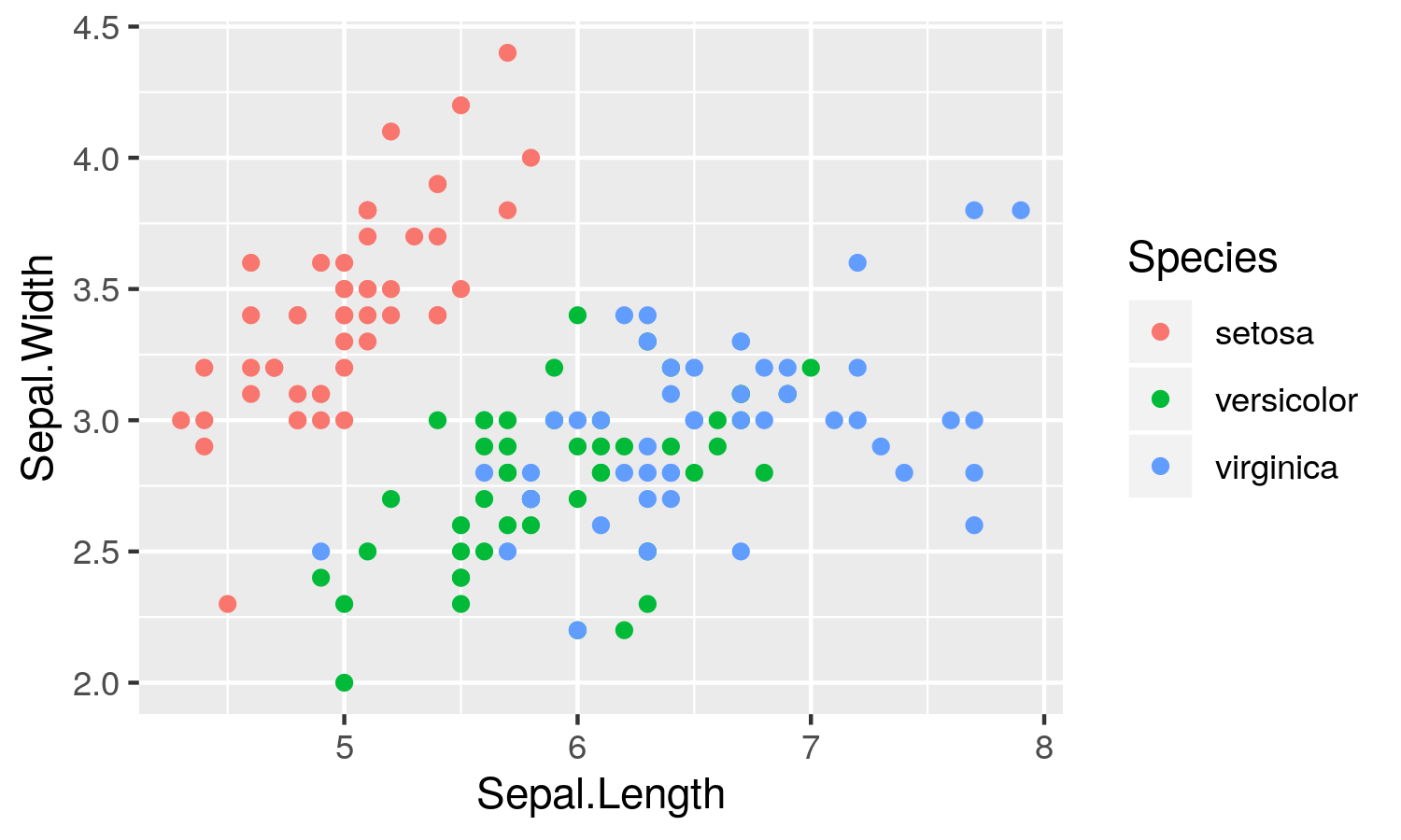<!-- --> ] - width and height of the plot in inches - Note that options are separated by commas --- # Chunk options ### What output each option suppresses? Option | Run code | Show code | Output | Plots | Messages | Warnings -------------------|:--------:|:---------:|:------:|:-----:|:--------:|:-------: `eval = FALSE` |<i class="fas fa-times "></i>| |<i class="fas fa-times "></i>|<i class="fas fa-times "></i>|<i class="fas fa-times "></i>|<i class="fas fa-times "></i> `include = FALSE` | |<i class="fas fa-times "></i>|<i class="fas fa-times "></i>|<i class="fas fa-times "></i>|<i class="fas fa-times "></i>|<i class="fas fa-times "></i> `echo = FALSE` | |<i class="fas fa-times "></i>| | | | `results = "hide"` | | |<i class="fas fa-times "></i>| | | `fig.show = "hide"`| | | | <i class="fas fa-times "></i>| | `message = FALSE` | | | | |<i class="fas fa-times "></i>| `warning = FALSE` | | | | | |<i class="fas fa-times "></i> Table from [R for Data Science](https://r4ds.had.co.nz/r-markdown.html#chunk-options) --- # Global chunk options ## Setup You can change the default chunk options for all following chunks in your document. ````md ```{r include = FALSE} knitr::opts_chunk$set( collapse = TRUE, cache = TRUE, comment = "#>", fig.width = 6, fig.align = "center" ) ``` ```` --- # <i class="fas fa-gamepad "></i> Exercice ## Let's practice ! 1. Open a new `.Rmd` document and run `data(diamonds)` within a chunk 2. Add the following text and fill it: ` We have data about XXXX diamonds. Only XXXX are larger than 2.5 carats. ` 3. Display all diamonds larger than 2.5 carats with the function `DT::datatable()`. 4. Make an histogram of the carats. The figure should have an height and width of 4 inches. 5. `DT::datatable()` doesn't work with PDF or Word document, why? <div class="countdown" id="timer_5da1c2fe" style="right:0;bottom:0;" data-warnwhen="0"> <code class="countdown-time"><span class="countdown-digits minutes">10</span><span class="countdown-digits colon">:</span><span class="countdown-digits seconds">00</span></code> </div> --- # Wrapping up ✔️ **Document your document**: use YAML to set up meaningful metadata ✔️ **Style your document**: use YAML to add options to your chosen output format ✔️ **Organize your text**: use markdown headers with `#` ✔️ **Organize your code**: use `knitr` chunk labels ✔️ **Style your text**: use markdown **bold**, *italics*, <i class="fas fa-list-ul"></i> bullets, and <i class="fas fa-list-ol"></i> lists ✔️ **Style your output**: use `knitr` chunk options 🧶 early, 🧶 often --- # Why using it? <i class="fas fa-arrow-circle-right "></i> Multiplateform | Portable | Reproducible <img src="assets/img/rmarkdownflow.png" width="100%" /> -- <i class="fas fa-arrow-circle-right "></i> Impress your director with dynamic output | Turn into a geek | Expose your skills on the web --- class: inverse, center, middle # <i class="fas fa-rocket "></i> Launch document on the web <html><div style='float:left'></div><hr color='#ffdd55' style="margin-top: -60px;" size=1px width=720px></html> --- # <i class="fas fa-rocket "></i> Launch document on the web ## Mission Send an HTML output on Github <img src="assets/img/rmarkdownflow_withSel_github.png" width="100%" /> --- # <i class="fas fa-rocket "></i> Launch document on the web ### 5 steps 1. Open new GitHub repository and activate Github page 2. Link this new repo to a RStudio project 3. Add a `.Rmd` document and generate the HTML document (we know that part!) 4. Declare (`add`) and document (`commit`) the modifications on the repository 5. Send these modifications with the HTML output on Github via RStudio -- ### Let's do it together! --- # <i class="fas fa-rocket "></i> Launch document on the web ### 1a. Open a new GitHub repository <img src="assets/img/createRepo.png" width="100%" /> -- - Name it as `firstOnlineDocument` - Let's make the repository public --- # <i class="fas fa-rocket "></i> Launch document on the web ### 1b. Activate Github page <img src="assets/img/config.png" width="100%" /> --- # <i class="fas fa-rocket "></i> Launch document on the web ### 1b. Activate Github page <img src="assets/img/gh-pages.png" width="100%" /> --- # <i class="fas fa-rocket "></i> Launch document on the web ### 1b. Activate Github page Several options <img src="assets/img/gh-pages_options.png" width="100%" /> --- # <i class="fas fa-rocket "></i> Launch document on the web ### 2. Link this new repo to a RStudio project In RStudio: file > new project... > Version control > Git <img src="assets/img/createProject.png" width="40%" style="display: block; margin: auto;" /> - Fill the field `Repository URL` with the URL address of your repo **and add `.git` at the end** - Exemple: `https://github.com/SteveViss/firstOnlineDocument.git` --- # <i class="fas fa-rocket "></i> Launch document on the web ### 3. Add a `.Rmd` document and generate the HTML document - You know that part, so let's do it. - We want to create a `.Rmd` and produces a `.html` file in the RStudio project folder. - <i class="fas fa-exclamation-triangle "></i> with the following filenames: `index.html` & `index.Rmd` - Make sure you save the files within the project folder <div class="countdown" id="timer_5da1c5cd" style="right:0;bottom:0;" data-warnwhen="0"> <code class="countdown-time"><span class="countdown-digits minutes">05</span><span class="countdown-digits colon">:</span><span class="countdown-digits seconds">00</span></code> </div> --- # <i class="fas fa-rocket "></i> Launch document on the web ### 4. Declare (`add`) and document (`commit`) the modifications on the repository <img src="assets/img/git1.png" width="100%" style="display: block; margin: auto;" /> --- # <i class="fas fa-rocket "></i> Launch document on the web ### 4. Declare (`add`) and document (`commit`) the modifications on the repository <img src="assets/img/git2.png" width="6936" height="80%" style="display: block; margin: auto;" /> --- # <i class="fas fa-rocket "></i> Launch document on the web ### 5. Last step, send these modifications on the Github repo via RStudio <img src="assets/img/git3.png" width="6936" height="80%" style="display: block; margin: auto;" /> --- # <i class="fas fa-rocket "></i> Launch document on the web Wait few minutes and see the result at [https://YOURUSERNAME.github.io/firstOnlineDocument/](https://YOURUSERNAME.github.io/firstOnlineDocument/) <img src="assets/img/ironcat.jpg" width="35%" style="display: block; margin: auto;" /> --- # <i class="fas fa-book "></i> The `down` universe - Write a notebook: `bookdown` - Write a thesis: `thesisdown` - Write a scientific article `rticles` - Create a poster: `posterdown` - Create nice presentation: `xaringan` or `rmarkdown` - Build a CV: `vitae` - Generate a blog: `blogdown` - Generate R package documentation: `pkgdown` --- class: inverse, center, middle # <i class="fas fa-rocket "></i> Building a presentation <html><div style='float:left'></div><hr color='#ffdd55' style="margin-top: -60px;" size=1px width=720px></html> --- # Motivation 1. Create a presentation <i class="fas fa-microphone "></i> 2. Use Markdown to quickly format your content 3. Insert code examples <i class="fas fa-cogs "></i> 4. Insert your R figures <i class="fas fa-chart-bar "></i> --- # Create a Rmarkdown presentation ## Templates in R Studio - [ioslides](https://bookdown.org/yihui/rmarkdown/ioslides-presentation.html) - [slidy](https://bookdown.org/yihui/rmarkdown/slidy-presentation.html) - also "r presentations" but it uses a different markdown syntax so we won't present it here <img src="assets/img/ioslides1.png" width="49%" /><img src="assets/img/ioslides2.png" width="49%" /> --- # Create a Rmarkdown presentation in R Studio .center[ 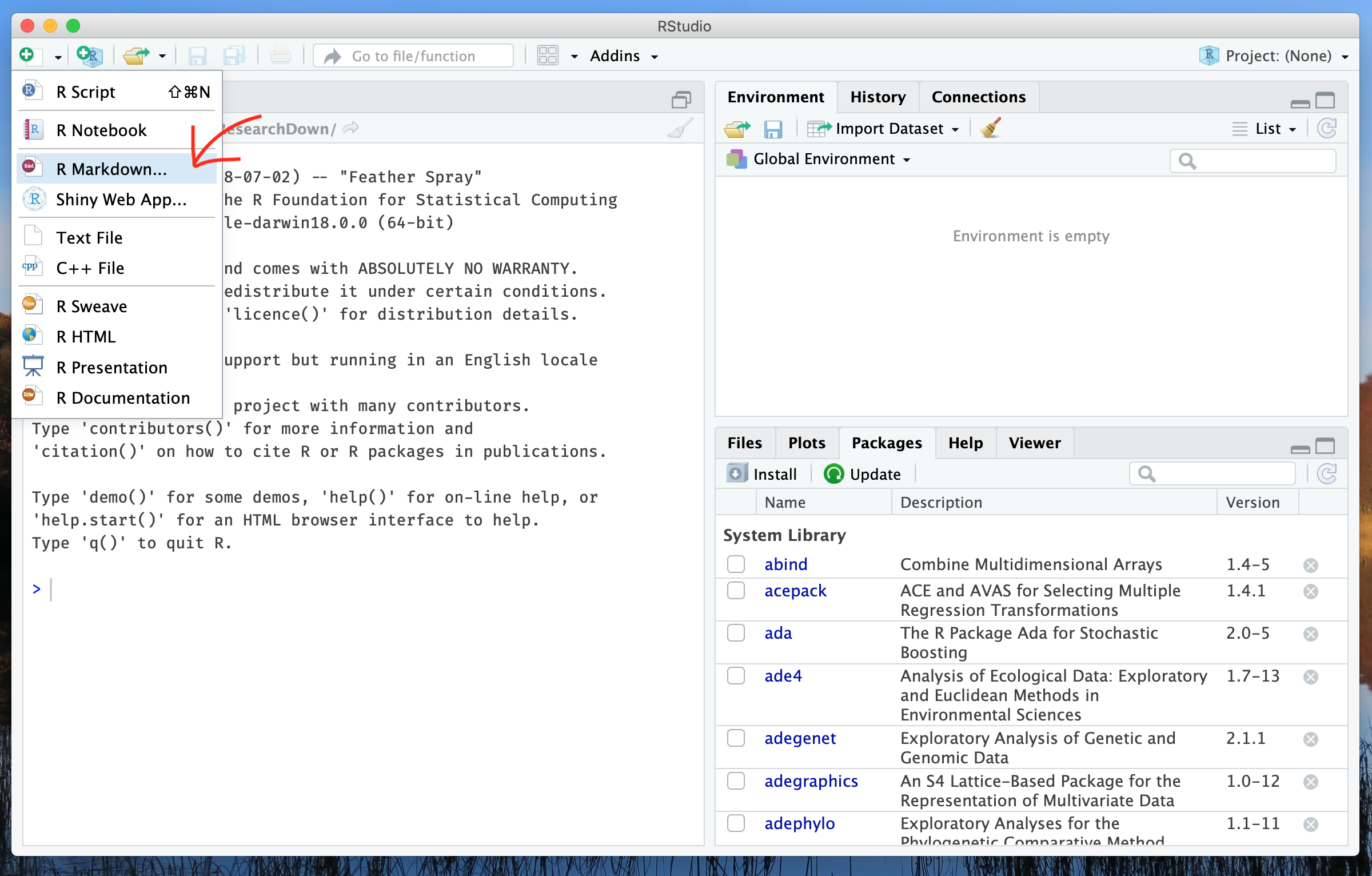 ] --- # Create a Rmarkdown presentation in R Studio .center[ 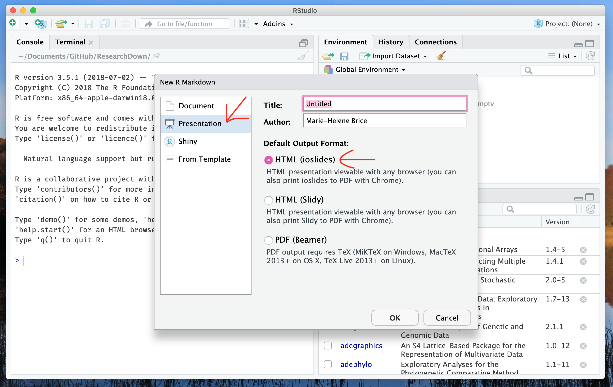 ] --- # ioslides Specify the `ioslides_presentation` output format in the YAML metadata of your document ```md --- title: "My beautiful ioslide presentation" author: "John Doe" date: '2019-10-02' output: ioslides_presentation --- ``` --- # ioslides Knit 🧶 to create the HTML presentation! .center[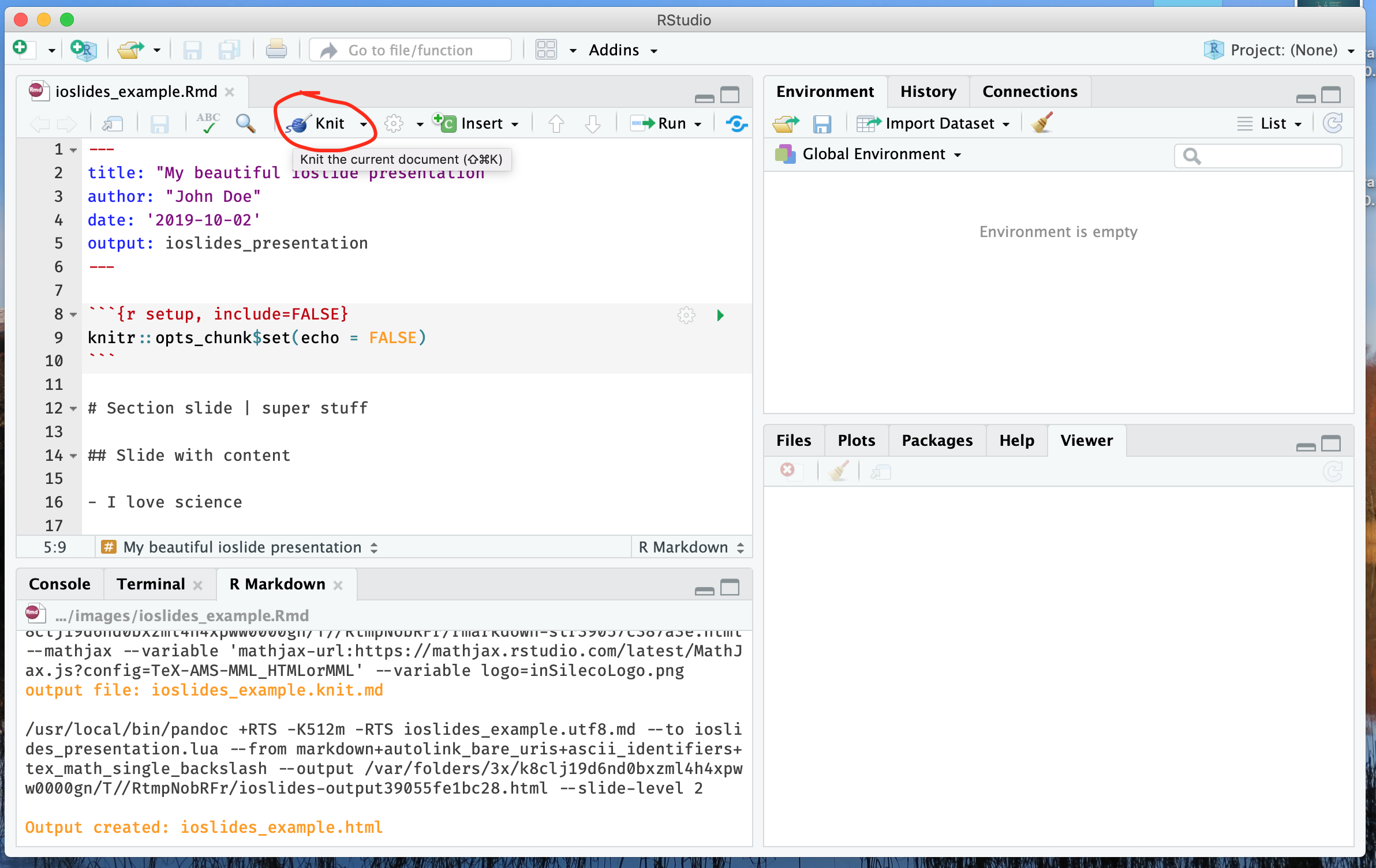] --- # ioslides Create new slides by using `#` or `##` ```md # Section slides | super stuff ``` .center[] --- # ioslides Create new slides by using `#` or `##` ```md # Section slide | with background image {data-background=bg_mountain.jpg data-background-size=cover} ``` .center[  ] --- # ioslides Create new slides by using `#` or `##` ```md ## Slides with content - I love science - and **kitten!** { width=60% } ``` .center[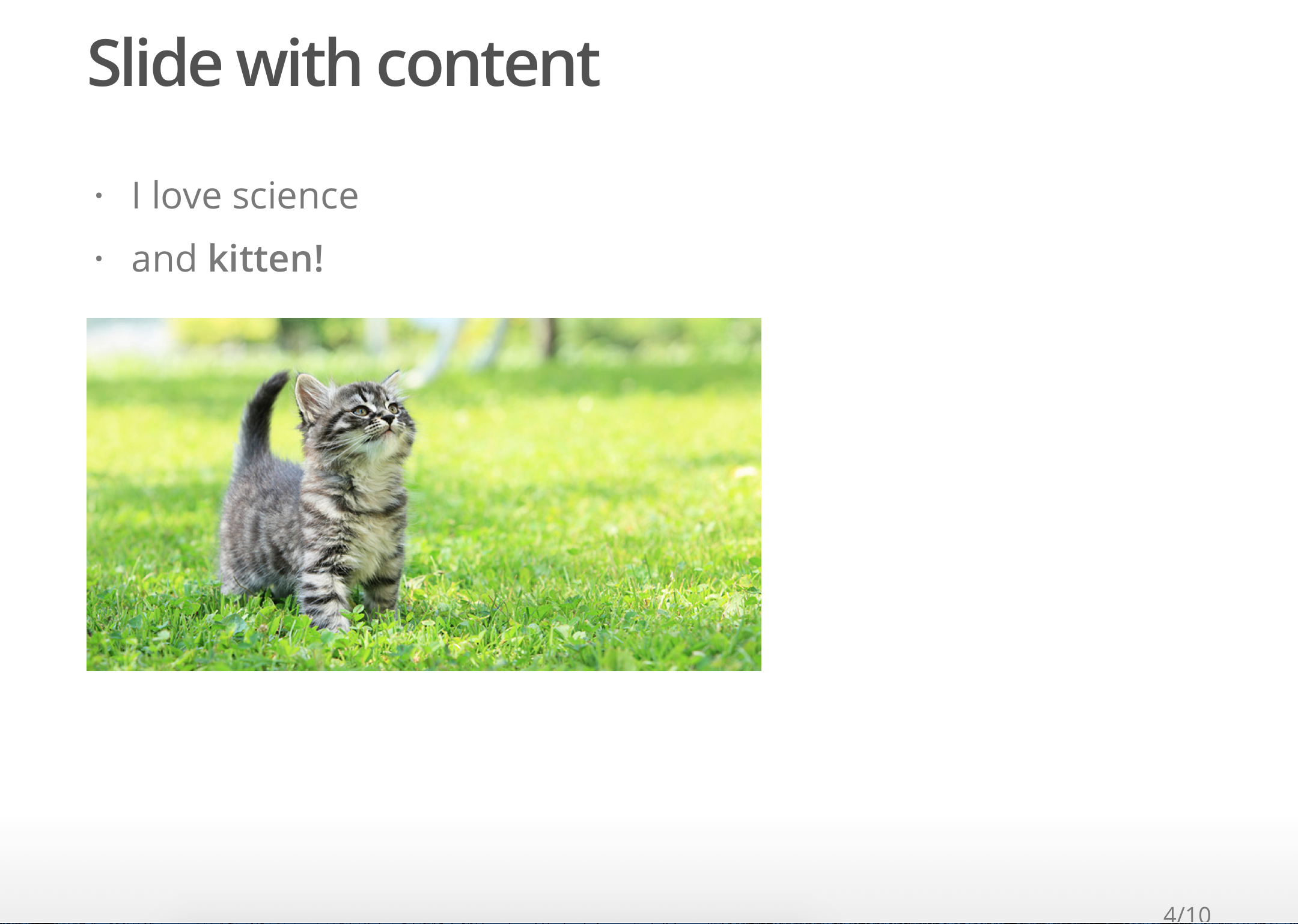] --- # ioslides - <i class="fab fa-r-project "></i> code ````md ## Slide with R code ```{r, echo = TRUE} fit <- lm(dist ~ 1 + speed, data = cars) coef(summary(fit)) ``` ```` .center[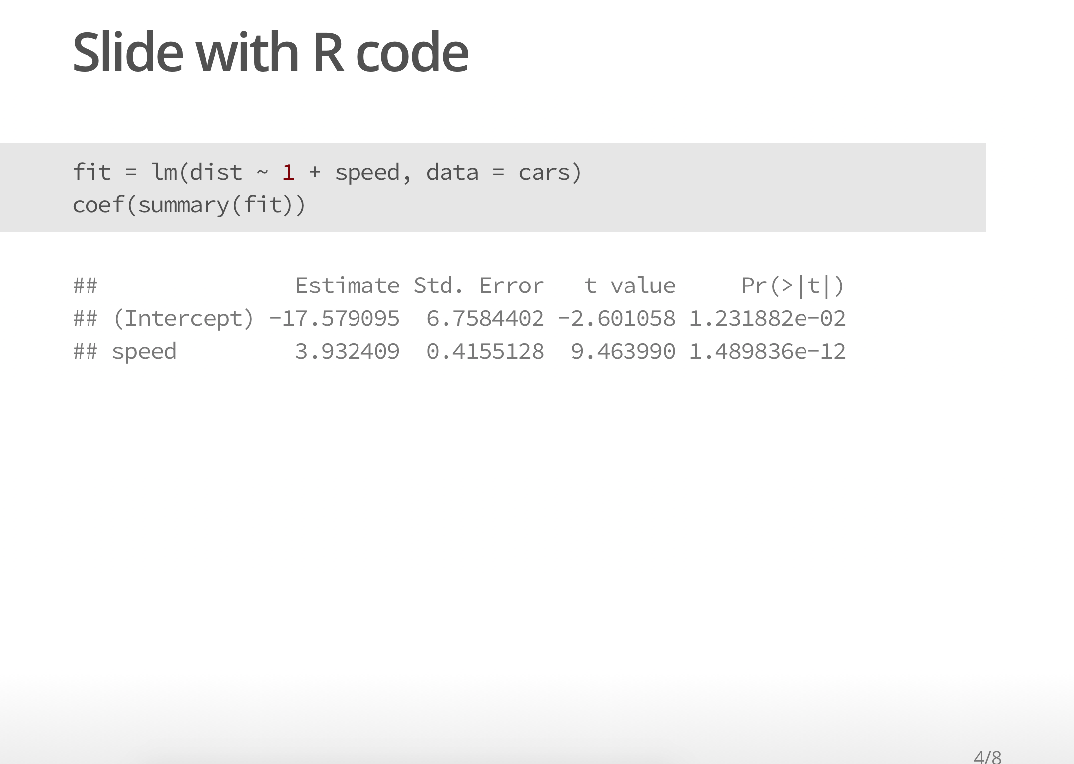] --- # ioslides - <i class="fab fa-r-project "></i> plot ````md ## Slide with R plot ```{r, echo = TRUE} plot(dist ~ speed, data = cars) ``` ```` .center[ 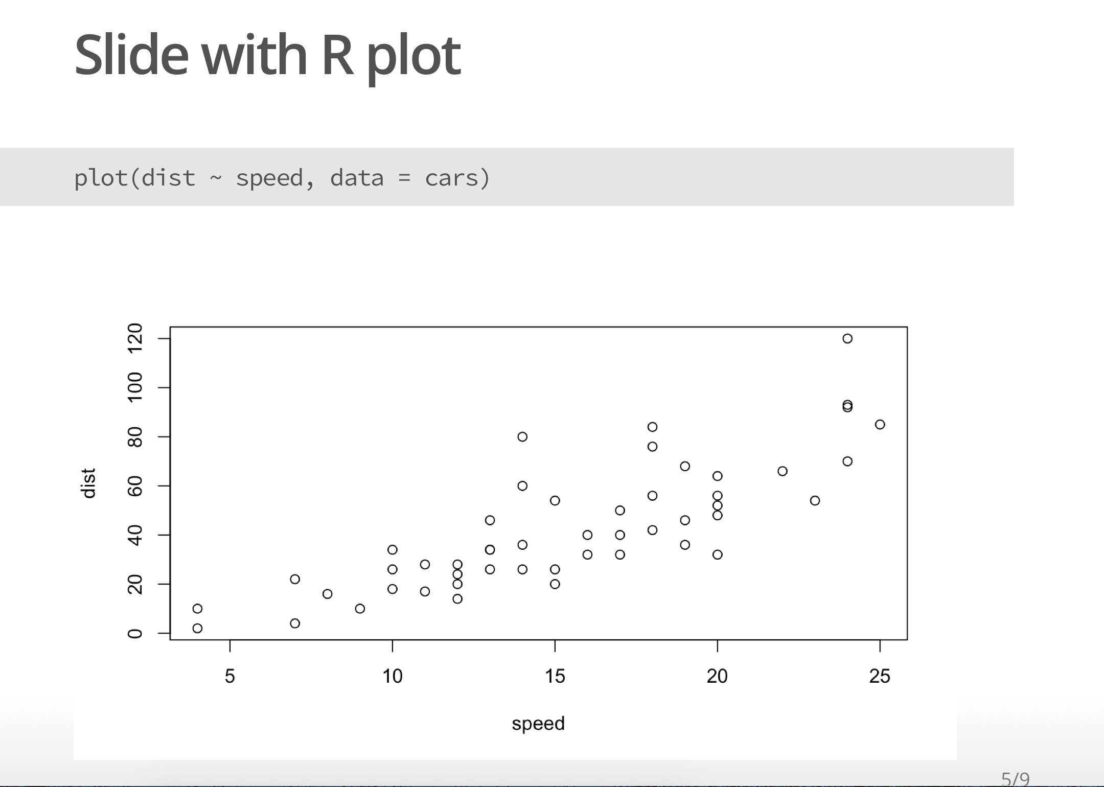 ] --- # ioslides - options ```md --- title: "My beautiful ioslide presentation" author: "John Doe" date: '2019-10-02' output: ioslides_presentation: logo: insilecoLogo.png --- ``` .center[ 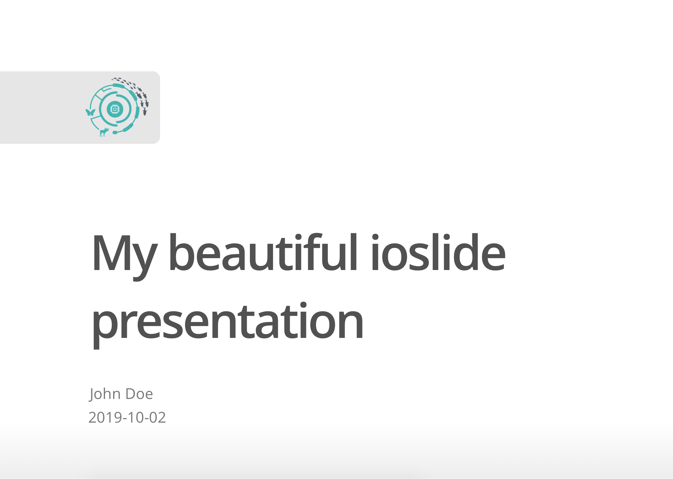 ] --- # ioslides - options ### Customize - presentation size using `widesreen` - speed of slide transitions using `transition` - incremental bullets using `incremental` - text size using `smaller` ```md --- title: "My beautiful ioslide presentation" author: "John Doe" date: '2019-10-02' output: ioslides_presentation: widescreen: true transition: slower incremental: true smaller: true --- ``` --- # ioslides - Customization You can customize your presentation by adding your own CSS and your own template ```md --- title: "My beautiful ioslide presentation" author: "John Doe" date: '2019-10-02' output: ioslides_presentation: css: mystyles.css template: mytemplate.html --- ``` --- # Slidy To create a [Slidy](https://bookdown.org/yihui/rmarkdown/slidy-presentation.html) presentation in R studio .center[ 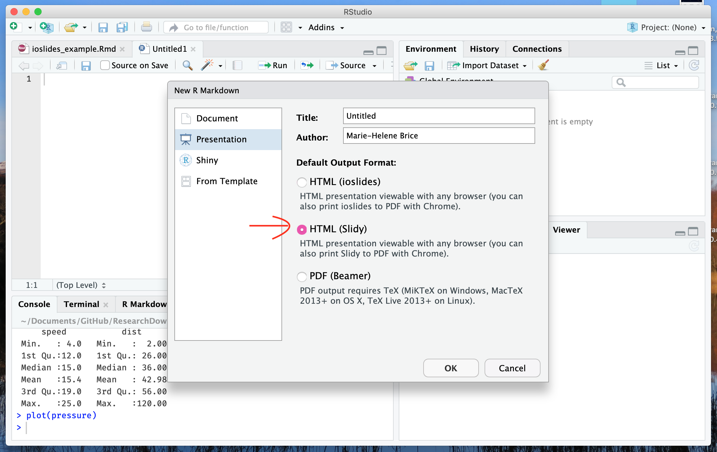 ] --- # Slidy - You can transform your ioslides presentation to a slidy presentation by changing the output format to `slidy_presentation` in the YAML - Usage of slidy is similar to ioslides, but see details [here](https://bookdown.org/yihui/rmarkdown/slidy-presentation.html) ```md --- title: "My beautiful slidy presentation" author: "John Doe" date: '2019-10-02' output: slidy_presentation --- ``` .center[ 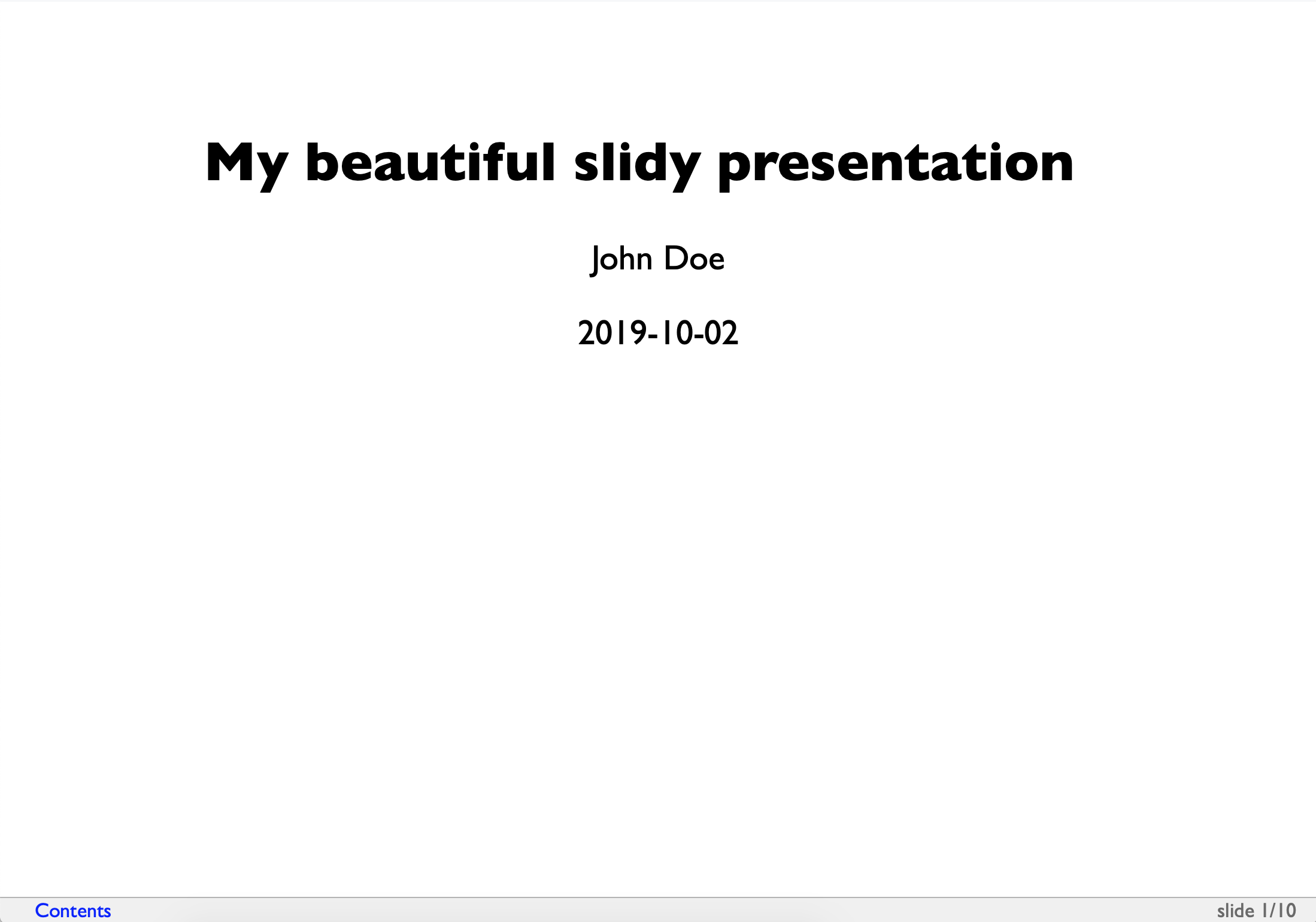 ] --- # PowerPoint - You can also generate a [PowerPoint](https://bookdown.org/yihui/rmarkdown/powerpoint-presentation.html) presentation using R! ```md --- title: "My beautiful PPT presentation" author: "John Doe" date: '2019-10-02' output: powerpoint_presentation --- ``` --- # Xaringan - It is also possible to install R packages to create presentation - ex: xaringan, see [here](https://slides.yihui.name/xaringan/#1) and [here](https://bookdown.org/yihui/rmarkdown/xaringan.html) ```r install.packages("xaringan") ``` ```md --- title: "My beautiful Xaringan presentation" subtitle: "Symposium" author: "John Doe" output: xaringan::moon_reader: --- # Slide 1 wow! --- # Slide 2 The end! ``` --- # Xaringan - QCBS R workshop presentations are built using xaringan! .center[ [](https://qcbsrworkshops.github.io/workshop01/workshop01-en/workshop01-en.html#1) ] --- # Resources 1. [R Markdown: The Definitive Guide - Chapter 4](https://bookdown.org/yihui/rmarkdown/presentations.html) 2. [ioslides](https://kevcaz.github.io/pres_Rmarkdown_fr/#1) 3. [xaringan](https://slides.yihui.name/xaringan/#1) --- class: inverse, center, middle # <i class="fas fa-rocket "></i> Create a notebook <html><div style='float:left'></div><hr color='#ffdd55' style="margin-top: -60px;" size=1px width=720px></html> --- # Motivation .pull-left[ - Producing more complicated documents - Automatic number and cross-referencing - Figures - Tables - Equations - Theorems - Custom headers - Figure formatting and placement - Customized visuals ] .pull-right[ <img src="https://bookdown.org/yihui/bookdown/images/logo.png" width="35%" style="display: block; margin: auto;" /> ] --- # With Rstudio project <img src="assets/img/bookdown_project.png" width="3729" height="60%" style="display: block; margin: auto;" /> --- # Bookdown - Examples - Minimal: https://bookdown.org/yihui/bookdown-demo/ <iframe width="100%" height="80%" src="https://bookdown.org/yihui/bookdown-demo/"> </iframe> --- # Bookdown - Examples - Tufte style: https://bookdown.org/yihui/bookdown-demo3/ <iframe width="100%" height="80%" src="https://bookdown.org/yihui/bookdown-demo3/"> </iframe> --- # Bookdown - Usage - Collection of `.Rmd` files - Individual chapter for each file - Chapter title defined by first-level heading `#` - Usual Rmarkdown syntax - Rendered by filename order by default .pull-left[ - `01-Introduction.Rmd` <br><br><br> - `02-Chapter1.Rmd` <br><br><br> - `03-Conclusion.Rmd` ] .pull-right[ ```r # Introduction This is the introduction ``` ```r # Chapter 1 This is the Chapter 1 ``` ```r # Conclusion This is the conclusion ``` ] --- # Bookdown - Usage - Outputs options - `HTML` - `pdf` - `E-Books` --- # Bookdown - Getting started <iframe width="100%" height="90%" src="https://bookdown.org/yihui/bookdown/get-started.html"> </iframe> --- # Bookdown - Resources - Github repository: https://github.com/rstudio/bookdown - Bookdown book: https://bookdown.org/yihui/bookdown/ --- # <i class="fas fa-book "></i> The `down` universe - Write a notebook: `bookdown` - Write a thesis: `thesisdown` - Write a scientific article `rticles` - Create a poster: `posterdown` - Create nice presentation: `xaringan` or `rmarkdown` - Build a CV: `vitae` - Generate a blog: `blogdown` - Generate R package documentation: `pkgdown`